Abstract
When fault such as pit failure arises in the rolling element bearing the vibration signal of which will take on periodic characteristics, and the abrupt failure of rotating machinery can be avoided effectively if the weak periodic characteristics of the early fault stage is extracted timely. However, the periodic characteristics of bearing’ early weak fault is hard to be extracted usually and the reasons can be boiled to as following: Firstly, the weak periodic signal of rolling element bearing’ early fault stage is buried by the strong background noise. Secondly, the weak fault cannot show the complete shock attenuation impulsive characteristic due to its weak energy, so the traditional wavelet transform would not work effectively if a proper wavelet basis function fitting for analyzing the impulsive characteristics is not selected. To solve the above two problems, a feature extraction method of the weak periodic signal of rolling element bearing’ early fault based on Shift Invariant Sparse Coding (SISC) originating from sparse representation is proposed in the paper. To capture the underlying structure of machinery fault signal, SICS provides an effective basis functions learning scheme by solving the flowing two convex optimization problems iteratively: 1) L1-regularized least squares problem. 2) L2-constrained least squares problem. The fault feature can be probably contained and extracted if optimal latent component is filtered among these basis functions. The feasibility and effectiveness of the proposed method are verified through the corresponding simulation and experiment.
1. Introduction
There are safe and economic significances in extracting the fault feature of rolling element bearing opportunely for its wide range using in rotating machinery. The traditional and classical techniques such as Fast Fourier Transform (FFT) and envelope demodulation (ED) were used for the purpose usually. However, the above two classical methods do not work effectively with the increasing complexity of the rotating machinery because the collected fault signal is becoming more and more complex. It is hard to diagnose the early weak fault of rolling element bearing and the corresponding technique is also a research hotspots. To solve the analyzed shortcomings of current fault diagnosis methods, a new fault diagnosis method of rotating machinery by combining wavelet packet decomposition (WPD) with empirical mode decomposition (EMD) was proposed in the paper [1]: the WPD was used as de-noising purpose and the EMD was used as fault feature extraction technique. The extract feature vectors were used as training and testing vector and input into the intelligent method, satisfactory classification result was obtained at last. The fault signal of rolling element bearing is easily overwhelmed by other strong vibration signals due to the close space locations of other vibration components in the machine. To solve the above problem, a new method named cyclic spike detection was proposed in paper [2] and used in recovery of the weak bearing fault features from a multi-component signal. The effectiveness of the proposed method in detecting cyclic spike was validated by the multi-components signal, including a simulated signal and a real vibration signal collected from an industrial machine. In paper [3], the minimum variance cepstrum (MVC) was used for detecting the periodic fault signal caused by the early fault of automotive ball bearing under running condition, and the analyzed results verify that feature of bearing’ early weak fault not only could be extracted effectively by the proposed method but also the proposed method is more advantage over other relative method such as cepstral. By combing discrete wavelet transform (DWT) with artificial neural network (ANN), a pattern classification method was proposed in paper [4]: The DWT was used as feature extraction method of the spur bevel gear box firstly. Then the extracted feature vectors were used as the training and testing input of the intelligent classification method (ANN), and satisfactory classification results were obtained at last. The two common used de-noising methods (wavelet decomposition-based de-noising and wavelet filter-based de-noising) were compared in paper [5], and the comparison results revealed that the latter is more suitable to detect the weak signature of mechanical impulse-like defect signals, whereas the former can achieve satisfactory results on smooth signal detection. Besides, the study on the selection of optimal parameters for wavelet filter was also carried out in the paper. An integrated method combing resonance demodulation with entropy threshold de-noising of wavelet packet coefficients was proposed in paper [6] to solve the difficulty of fault feature extraction of the early weak impulsive signal. The validity and effectiveness of the proposed method in feature extraction of rolling element bearing’ early weak impulsive signal were proved by the analysis results of experiment data. The virtues of tunable Q-factor wavelet transform (TQWT) and neighboring coefficient de-noising were combined in paper [7] to propose a de-nosing method of the rolling element bearing’ early weak fault signal corrupted by strong background noise. The experiment results demonstrated that the proposed method can identify the fault features much more successfully than other conventional wavelet thresholding de-noising methods. In paper [8], The EEMD and tunable Q-factor wavelet transform methods are combined and used in fault diagnosis of rolling element bearing’ early weak fault successfully. Though considerable results are achieved, most of the above cited papers obtained the test damaged rolling element bearing with different size using electrical discharge machining (EDM) technology to simulate the early weak fault. In actual, it is a very complicated and long process from the installation of rolling element bearing to its natural ultimate failure, so it is not reasonable to process fault on the parts of rolling element bearing using EDM directly. In this paper, the rolling element bearing accelerated life test is carried out to obtain the vibration data of the testing bearings’ three stages: The data of their installation stage, their fault initial stage and their final failure stage. The effectiveness and feasibility of the proposed method are verified by using the vibration data of the bearings’ initial stage.
SISC [9, 10] is a new signal processing method based on sparse representation, and its application in fault diagnosis of rotating machinery’ weak fault is very limited. In paper [11] a redundant dictionary from a large number of existing signals was trained using SISC, and the classification of different kinds of bearing faults was realized at last. From a different perspective, the basic idea of this paper is to penetrate into the underlying structure of the signal to realize noise cancellation and feature extraction. SISC is used here as the basis function learning algorithm to capture different structural characteristics hided in the signal. By decomposing the original signal into these basis functions simultaneously, fault related time series can be separated through optimal latent component filtering. So, the method proposed in this paper can be considered as a feature enhancing technique without requiring any prior knowledge.
The paper is organized as following: The theories of sparse representation and SISC are presented roughly in Section 2. In Section 3, the processes of SISC in feature extraction of the weak periodic signal of rolling element bearing’ early fault are given. Section 4 is the simulation to verify the effectiveness of the proposed method. In Section 5 the analyzed results of the experimental data using the proposed method are presented. The contents in Section 6 dedicate the conclusions obtained from the above results.
2. SISC
2.1. Sparse representation
The idea of decomposing signal with the over-complete dictionary of atoms on basis of wavelet transform was put forward by Mallat and Zhang. The common used over-complete dictionary taking wavelet dictionary, Gabor dictionary, wavelet dictionary and so on for example is over-complete which is composed of numbers of atoms. The original signal is represented by using atoms as few as possible in the sparse mode:
is the analyzed discrete-time signal in the above equation, and is a matrix also called redundant dictionary which can span the entire Hilbert space . The can be defined as the over-complete dictionary if there exists . The coefficients for each atom are represented as .
There are numerous of methods to the solution of in Eq. (1) for the reason of over-completeness. The preference is made towards the one with the minimum norm among the numbers of methods. The sparse decomposition is determined by:
The minimization of norm in Eq. (2) is a NP-hard problem which is difficult to solve. Therefore, alternative solutions such as MOF, BOB, MP, BP and so on are proposed basing on different strategies. The composition with minimum norm of the coefficients is chosen by MOF. BOB finds the orthogonal basis by minimizing the entropy measure of the coefficients. MP selects atoms by using a stepwise greedy approximation algorithm. BP selects the representation with minimum norm. Compared with other algorithms, BP has the advantages of better sparseness and accuracy. However, it suffers from slower computation speed. The comparisons of some main sparse decomposition algorithms are shown in Table.1. More generally, sparse coding poses the following optimization problem to compute the maximum-a-posteriori (MAP) estimation of both and :
There exists two issues in sparse representation as demonstrated in Eq. (3): 1) The solving of sparse coefficients. 2) The design of the redundant dictionary.
Table 1Comparison of sparse decomposition algorithms
Algorithms | Sparseness measurement | Sparseness of the solution result | Calculation speed | Accuracy |
CM | Optimal | Very slow | Very good | |
BP | Very good | Slow | Very good | |
MP | Sub or local optimal | Good | Moderate | Good |
FOCUSS | Very good | Slow | Very good | |
MOF | Not good | Very fast | Poor | |
IPM | Sub or local optimal | Good | Fast | Moderate |
BOB | Sub or local optimal | Good | Fast | Moderate |
2.2. SISC model
The model of SISC can be represented as shown in Eq. (4) which is different from the traditional sparse representation model as shown in Eq. (1):
where the basis function , can be replicated at each time offset within the signal and they can appear at all possible shifts. Any signal , could be encoded with a set of basis functions. Each basis function being used at all possible time shifts within is represented by the convolution operator * succinctly. The main difference between the models of SISC and sparse representation is that the basis functions of the former are allowed to be lower dimension than the input signal. Furthermore, the coefficients is a vector and the size of which is . The learning of basis functions and coefficients under the maximum-a-posteriori can be solved by solving the following optimization problem:
The value of is prevented from becoming too large by the constrain shown in Eq. (6). The objective function Eq. (5) is to convex one of and , so the solution of basis functionscan be realized by fixing the values of coefficients , and to solve the by fixing .
2.3. SISC algorithm
The optimization problem shown in Eq. (5) can be attributed to a very large sparse representation problem like Eq. (3) with tied parameters by expanding out the convolution. However, even moderate problem sizes will be infeasible to solve due to the reason that the reformulation would ignore the special structure in the Eq. (5). An efficient SISC algorithm will be introduced and used in the paper.
The solution of sparse coefficients is a regularized least squares problem if the basis function is fixed, and the problem can be reduced to an unconstrained quadratic optimization problem using feature-sign search algorithm [9]. Keeping the sparse coefficients fixed, and the solution of reduces the objective function Eqs. (5) and (6) into a constrained optimization problem:
Different components of basis functions will be coupled in the objective because each basis function can appear in any possible shift and each component of the basis function vector contributes to many different terms in the objective function. The solution to the above problem can turn to be transformed into the frequency domain because the convolution can be replaced by product:
The discrete Fourier transforms of the basis function and input signal in Eq. (9) are represented by and respectively. The Parseval’s theorem is the theoretical guarantee of from Eq. (7) to Eq. (10), which proves that the discrete Fourier transform scales the norm by a constant factor . So, Eq. (9) and Eq. (10) are equivalent to the optimization problem with regard to Eq. (7) and Eq. (8), because their objective and constrains both consist of terms. A sum of quadratic terms can be obtained by decomposing the lagrangian to solve the problem, and each quadratic term depends on a single frequency component :
with dual variables , unit vector , and:
Though it is hard to obtain the most optimal result in Eq. (11), it can be expressed as a function of only real variables using real and imaginary parts of. The obtaining of can be realized by optimizing over and :
The detailed optimization processes can be referred to paper [10].
3. The flow chart of the proposed method
The time-domain waveform of the vibration signal will take on periodic impulsive characteristics when pitting failure arises in any parts (inner race, outer race or rolling elements) of the rolling element bearing. These periodic shocks have the same structure usually because they are produced by the same failure location. The reasonable way is that the periodic shocks may be represented by just one basis function, and the SISC algorithm is very fit for analyzing the fault vibration signal:
1) The periodic shocks repeating in the fault vibration signal can be expressed by one basis function because anyone basis function in the SISC function dictionary can be moved to any position in the time-domain through time-shifting method.
2) The basis functions in the SISC method are obtained through self-learning type, so it is much more self-adapting than the traditional sparse representation and wavelet transform methods.
The overall flow chart of the proposed method is shown in Fig. 1 which can be divided into two steps mainly:
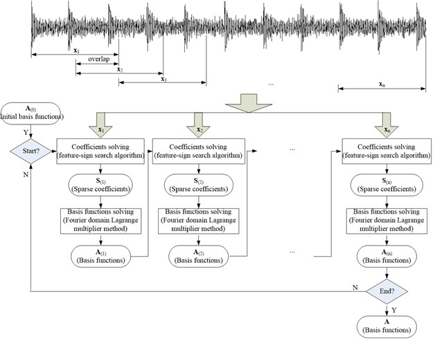
Step 1: Fault feature learning from machinery fault signal: The access of the redundant dictionary usually requires a set of standard training signals through learning. However, there is not so called standard training samples due to the difference of equipment type and operation condition. A more effective and practical method is to use the signal itself as the training sample to obtain the dictionary. The specific processes are given in Fig. 2, and the process of OMP (Orthogonal Matching Prusuit) and UCLDA (Union of Circulants Dictionary Learning Algorithm) can be referred to paper [12, 13].
Step 2: Optimize latent component filtering, and the specific processes are given in Fig. 3.
Fig. 1The overall flow chart of the proposed method
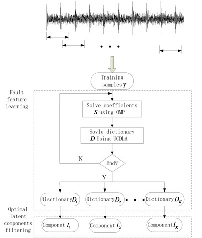
Fig. 2Feature learning
4. Simulation
The mathematical equation of rolling bearing fault model can be expressed as Eq. (13) [14, 15] and is used to verify the feasibility of the proposed method. In Eq. (13), is the tiny fluctuation around mean period . Set the sampling frequency 25600 Hz, and the shaft rotation frequency is 8 Hz. The inner race and outer race fault characteristic frequencies are 60 Hz and 48 Hz respectively. Assuming the random slide between rolling element and race is normally distributed whose standard deviation is 2 % of the shaft rotation ratio:
Fig. 3Optimal latent component filtering
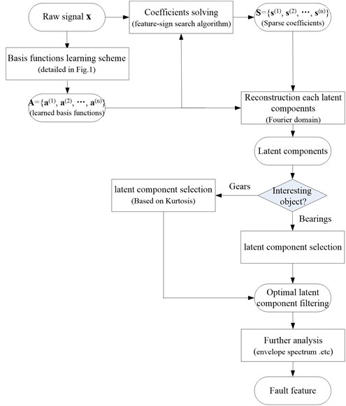
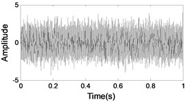
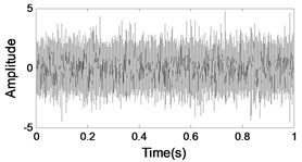
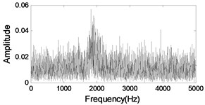
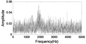
Fig. 4Simulation signal: a) time waveform for outer race fault, b) frequency spectrum for outer race fault, c) time waveform for inner race fault, d) frequency spectrum for inner race fault
a)
b)
c)
d)
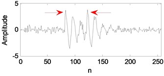
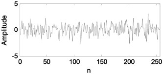
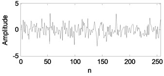
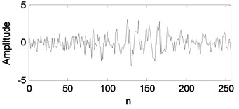
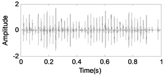
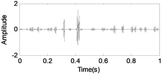
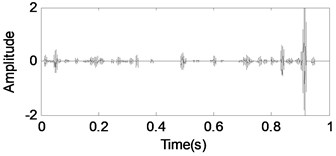
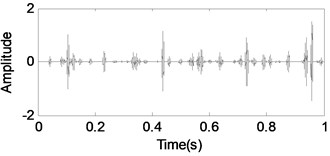
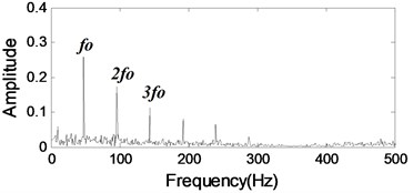
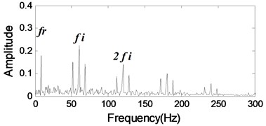
The time-domain waveforms of the outer race and inner race simulation fault signals are shown in Fig. 4(a) and (c) respectively and their corresponding frequency-domain waveforms are shown in Fig. 4(b) and (d). The analyzed results of the outer race fault simulation signal based on the proposed method as shown in Fig. 2 and Fig. 3 are shown from Figs. 5-7: As shown in Fig. 5, there are four learned basis atoms of the outer race fault simulation signal as shown in Fig. 4(a). The four reconstructed component of bearing outer race fault simulation signal are shown in Fig. 6. The constructed component shown in Fig. 6(a) owns the proper periodic impulsive characteristics, and its corresponding envelope demodulation spectrum is shown in Fig. 7 from which the outer race fault characteristic frequency and its harmonic frequencies are extracted perfectly.
Fig. 5The four learned basis atoms of bearing outer race fault signal: a) d1, b) d2, c) d3, d) d4
a)
b)
c)
d)
Fig. 6The four reconstructed component of bearing outer race fault signal: a) l1, b) l2, c) l3, d) l4
a)
b)
c)
d)
Fig. 7The envelope spectrum of l1
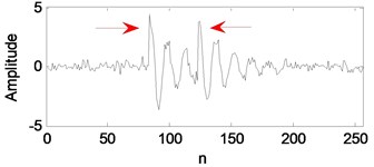
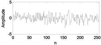
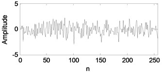
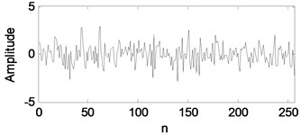
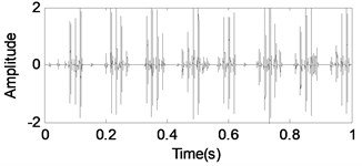
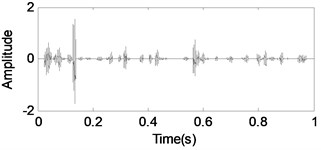
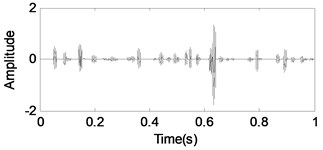
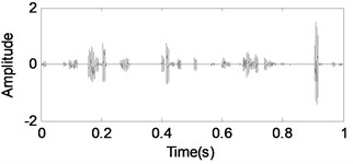
The analyzed results of the inner race fault simulation signal are shown in Figs. 8-10, and the meanings of each figure are same as the figures shown in Figs. 5-7.
Fig. 8The four learned basis atoms of bearing inner race fault signal: a) d1, b) d2, c) d3, d) d4
a)
b)
c)
d)
Fig. 9The four learned reconstructed component of bearing inner race fault signal: a) l1, b) l2, c) l3, d) l4
a)
b)
c)
d)
Fig. 10The envelope spectrum of l1
5. Experiment
Though different kinds of rolling element bearing faults can be simulated by EDM technique to study the corresponding fault diagnosis methods, the early weak fault of rolling element bearing is hard to obtain or simulate by EDM technique because the process of rolling element bearing’ whole life is very complex and long under normal conditions. In order to study the fault diagnosis technique of the rolling element bearing’ early weak, the accelerated bearing life test (ABLT-1A) is carried out in the paper. The test rig is shown in Fig. 11 which can host four testing rolling element bearings simultaneously. Vibration data is collected by three acceleration sensors and the installation sketch of them is shown in Fig. 12. Besides, the force shown in Fig. 12 is enforced in order to accelerate the whole life test. The parameters of the testing bearing are shown in Table 2 and the corresponding theory fault characteristic frequencies are shown in Table 3. In Table 3 represents the rotating frequency of the rolling bearing, and is the fault characteristic frequency of the rolling bearing cage., and are the fault characteristic frequencies of rolling bearing’ rolling element, inner race and outer race respectively. One group of 20480 points is collected per minute and the sampling rate is set as 25.6 kHz. Continue the experiment until there is fault arising in any one of the four bearings (stop the experiment when there is evident vibration occurring in the test rig). The RMS (root mean square) values of the four test bearings (B1, B2, B3 and B4) as shown in Fig. 12 over their whole life (There are 1263 groups data in all) are shown in Fig. 13: The RMS values of B1 and B2 are almost unchanged which verifies that there are not faults arising in B1 and B2, and the disassemble of B1 and B2 after experiment verifies their intact conditions further. There is slight fluctuation of the RMS values of B4 over its whole life and this phenomenon can be explained by the self-healing theory of rolling element bearing: when very tiny pitting fault arises in rolling element bearing, the weak fault will be healed by the continuous collision rolling body.
Fig. 11The schematic diagram of the experiment equipment
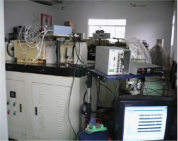
Fig. 12The sketch of acceleration sensors installation
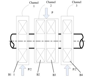
Table 2The parameters of the test rolling bearing
Type | Ball number | Ball diameter (mm) | Pitch diameter (mm) | Contact angle | Motor speed (rmp) | Load (kN) |
6307 | 8 | 13.494 | 58.5 | 0 | 3000 | 12.744 |
Table 3The fault characteristic frequencies of the test rolling bearing
50 | 19 | 102 | 246 | 153 |
There are obvious changes of the RMS values of B3 over its whole life which shows that there is fault arising in it, and there is obvious fault arising in the inner race (The inner race fault is shown in Fig. 14) of B3 after disassemble of it when the experiment is over. As shown in Fig. 13, the RMS values of B3 are almost unchanged before the 1210th group. The 1211th-1263th can be considered as the evident fault occurring stage. It will be meaningful to avoid serious failure if the fault characteristic can be extracted successfully before the 1210th group. The 1116th group data of B3 is used to verify the effectiveness of the proposed method.
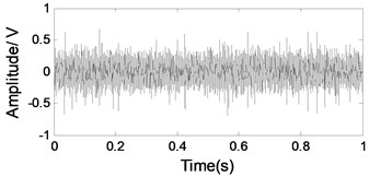
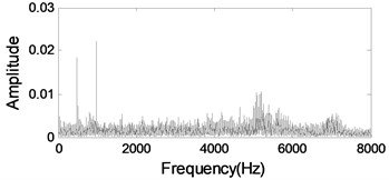
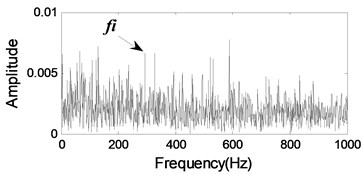
The time-domain waveform of the 1116th group data is shown in Fig. 15(a) and its corresponding frequency spectrum and envelope spectrum are shown in Fig. 15(b) and Fig. 15(c) respectively: In the time-domain waveform there is not evident impulsive phenomenon and the weak periodic characteristic could not be identified.
Fig. 13The RMS value of four bearings
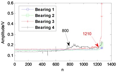
Fig. 14The inner race fault
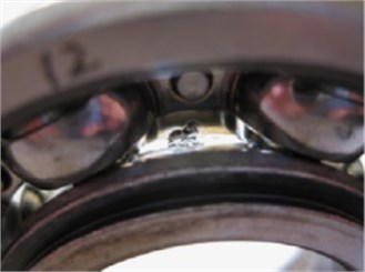
Fig. 15The 1116th signal for Bearing 3: a) time waveform, b) frequency spectrum, c) envelope spectrum
a)
b)
c)
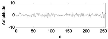
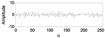
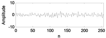
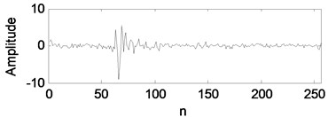
Fig. 16The four learned basis atoms: a) d1, b) d2, c) d3, d) d4
a)
b)
c)
d)
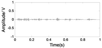
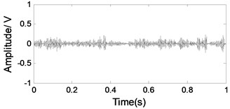
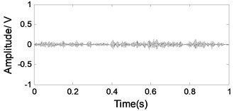
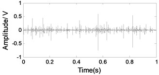
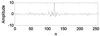
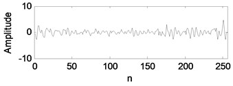
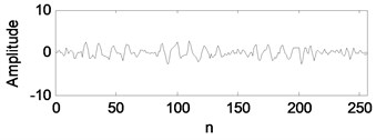
Besides, the analyzed results using the traditional signal processing methods such as FFT and envelope demodulation are shown in Fig. 15(b) and (c), and the results verify that the above two traditional methods also do not work. Apply the proposed method as shown in Fig. 2 and Fig. 3 on the early weak fault signal as shown in Fig. 15(a), and the analyzed results are shown from Fig. 16 to Fig. 18: In Fig. 16, the four learned basis atoms are presented, and the corresponding constructed four components are shown in Fig. 17. The envelope demodulation spectrum of the constructed component as shown in Fig. 17(d) is shown in Fig. 18 from which the inner race fault characteristic frequency with its harmonics are extracted successfully. The effectiveness of the proposed method is verified further through the analysis result of the early weak fault of B3.
Fig. 17The four learned reconstructed component: a) l1, b) l2, c) l3, d) l4
a)
b)
c)
d)
Fig. 18The envelope spectrum of l4
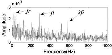
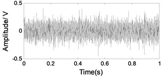
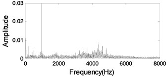
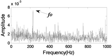
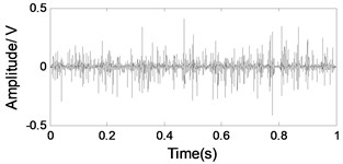
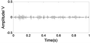
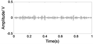
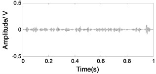
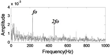
In Fig. 13, the RMS values of B4 change some bigger at the 800th group. Same as the analysis ideology and processes of B3, the analysis results of the 800th group data of B4 using traditional methods and the proposed methods are shown from Fig. 19 to Fig. 22. The time-domain waveform of the 800th group data of B4 is shown in Fig. 19(a), and its corresponding frequency-domain waveform and envelope spectrum are shown in Fig. 19(b) and Fig. 19(c). Though the outer race fault characteristic frequency could be extracted based on Fig. 19(b) and Fig. 19(c), the harmonic could not be extracted as shown in Fig. 22 using the proposed method.
Fig. 19The 800th signal for Bearing 4: a) time waveform, b) envelope spectrum
a)
b)
c)
Fig. 20The four learned basis atoms: a) d1, b) d2, c) d3, d) d4
a)
b)

c)
d)
Fig. 21The four learned reconstructed component: a) l1, b) l2, c) l3, d) l4
a)
b)
c)
d)
Fig. 22The envelope spectrum of l1
The above are the analysis results of the early weak fault signals of the accelerated bearing life test using the proposed method, and the analyzed signals are almost close to the result of the bearing’ natural degradation which is almost same as the actual engineering, so the results are much more convicted.
6. Conclusions
There are economy and security significances to study the fault diagnosis technique of rolling element bearing’ early weak fault to avoid the problems of excess or inadequate maintenance. Usually, the traditional signal processing methods such as Fast Fourier Transform (FFT) and envelope demodulation and so on could not extract the fault feature of rolling element bearing’ early weak fault successfully. By combining the periodic property of rolling bearing’ fault signal with the characteristic of SISC, a method of feature extraction of the weak periodic signal of rolling element bearing’ early fault based on Shift Invariant Sparse Coding is proposed in the paper. The proposed method can extract the feature of the repetitive arising weak fault signal successfully through the verification of simulation and experiment results. The proposed method provides a new solution for early fault detection of rolling element bearing. However, compound fault usually arises in the early fault stage of rotating machinery, and it is hard to diagnose the compound fault of rotating machinery compared to the single fault. Up to now, very limited papers relating to the diagnosis of rotating machinery’ compound fault arise, so it is necessary to carry out the corresponding studying of diagnosis of rotating machinery’ compound fault. There is great application potential of SISC in the area, so the authors will carry on the relative studying in the next step.
References
-
Bin G. F., Gao J. J., Li X. J. Early fault diagnosis of rotating machinery based on wavelet packets-empirical mode decomposition feature extraction and neural network. Mechanical System and Signal Processing, Vol. 27, 2012, p. 696-711.
-
Wang D., Guo W., Wang X. J. A joint sparse wavelet coefficient extraction and adaptive noise reduction method in recovery of weak bearing fault features from multi-component signal mixture. Applied Soft Computing, Vol. 13, 2013, p. 4097-4104.
-
Park C. S., Choi Y. C., Kim Y. H. Early fault detection in automotive ball bearings using the minimum variance cepstrum. Mechanical Systems and Signal Processing, Vol. 38, 2013, p. 534-548.
-
Saravanan N., Ramachandran K. I. Incipient gear box fault diagnosis using discrete wavelet transform (DWT) for feature extraction and classification using artificial neural network (ANN). Expert Systems with Application, Vol. 37, 2010, p. 4168-4181.
-
Qiu H., Jay L., Lin J., Yu G. Wavelet filter-based weak signature detection method and its application on rolling element bearing prognostics. Journal of Sound and Vibration, Vol. 289, 2006, p. 1066-1090.
-
Cui L. L., Kang C. H., Xu Y. G., Gao L. X. Integrated algorithm research on early impactive fault feature extraction of rolling beraring. Chinese Journal of Scientific Instrument, Vol. 31, 2010, p. 2422-2427.
-
He W. P., Zi Y. Y., Chen B. Q., Wang S., He Z. J. Tunable Q-factor wavelet transform denoising with neighboring coefficients and its application to rotating machinery fault diagnosis. Science China Technological Sciences, Vol. 56, 2013, p. 1956-1965.
-
Wang H. C., Chen J., Dong G. M. Feature extraction of rolling bearing’s early weak fault based on EEMD and tunable Q-factor wavelet transform. Mechanical Systems and Signal Processing, Vol. 48, 2014, p. 103-119.
-
Lee H., Battle A., Raina R., Ng A. Y. Efficient sparse coding algorithms. Advances in Neural Information Processing Systems, Vol. 19, 2007, p. 801-808.
-
Grosse R., Raina R., Kwong H., Ng A. Y. Shift-invariant sparse coding for audio classification. Proceedings of the 23rd Conference on Uncertainty in Artificial Intelligence, 2007.
-
Liu H. N., Liu C. L., Huang Y. X. Adaptive feature extraction using sparse coding for machinery fault diagnosis. Mechanical Systems and Signal Processing, Vol. 25, Issue 2, 2011, p. 558-574.
-
Labusch K., Erhardt B., Martinetz T. Demixing Jazz-music: Sparse coding neural gas for the separation of noisy overcomplete sources. Neural Network World, Vol. 19, Issue 5, 2009, p. 581-596.
-
Xiao B. Sparse and low-rank modeling on high dimensional data: a geometric perspective. Ph.D. Thesis, North Carolina State University, 2014.
-
Mcfadden P. D., Smith J. D. Model for the vibration produced by a single point defect in a rolling element bearing. Journal of Sound and Vibration, Vol. 96, Issue 1, 1984, p. 69-82.
-
Mcfadden P. D., Smith J. D. The vibration produced by multiple point defects in a rolling element bearing. Journal of Sound and Vibration, Vol. 98, Issue 2, 1985, p. 263-273.
