Abstract
One high fidelity numerical method is extended to compute the unsteady aerodynamic loads when micro rotary wings suffer wind. The unsteady solutions are obtained by solving Navier-Stokes equations, where field velocity method is proposed to carry out the atmospheric perturbation. The convective terms are approximated by a high order WENO-Roe scheme, and time advance is performed by an implicit scheme of dual time stepping which can guarantee a degree of efficiency. Moving overset grids are used to facilitate the implement of rotational motion of rotary wings and relative movements between rotary wings, as well as the atmospheric perturbation. The results reveal that small atmospheric perturbation has an important impact on the flows of micro rotary wings under low Reynolds number. The response of thrust coefficient presents periodic fluctuation and its amplitude is proportional to that of wind disturbance, which provides the clue for active control research of rotary wing aircraft.
1. Introduction
Due to the technological achievements made in modern flight in recent years, more and more attention has been paid to the unavoidable negative effects on the fatigue characteristics and flight quality of aircraft induced by gust response. In the practical engineering problems, sudden winds have a significant impact on the aeroelasticity and the aerodynamic noise of aircraft wings and turbofan, as well as helicopter rotor [1-3]. For micro aerial vehicles (MAV), they are expected to perform hovering flights as well as aggressive flights despite possible wind perturbation [4], which requires advanced control technology. However, before the corresponding control method is adopted, the unsteady aerodynamic loads should be accurately predicted when the aircraft suffers gust.
Simulation technique based on computational fluid dynamics (CFD) [5-12] is a very popular and important way to understand some assumptions on the gust loads and verify the accuracy of prediction. In the work of Parameswaran, Baeder and Singh et al. [8, 9], unsteady Euler/Navier-stokes solver was directly used to compute not only the indicial responses of an airfoil in regard to step changes in attack angle and pitch rate, but also the penetration of a sharp-edged gust through exerting perturbation to flow fields. For Euler/Navier-Stokes solvers, the gust disturbance input can be applied on the airfoil or wing as a boundary condition, but some problems maybe happen in the flow due to the infinite time derivative, such as numerical oscillations, numerical instability and nonphysical feature [8]. Sometimes, by using this method, the step input of one parameter may change another input parameter, which maybe results in the incorrect indicial response. One case is that if angle of attack of aircraft is suddenly changed, the airfoil would go through an infinite pitch rate, which shows that the step change of attach angel could lead to an impulsive phenomenon in the pitch rate. On the other hand, gust modeled by using grid velocity was a simple and effective method, which is essentially a field velocity method [7-12]. Although that velocity of the grid usually means the physical movement of the grid, it is possible to introduce an atmospheric perturbation velocity in a stationary grid by describing the grid velocity in some field grid points where the grid does not actually move. Recently, CFD based on a field velocity method of modeling gusts was adopted for a truss braced wing aircraft [11, 12]. The results showed that the method has the advantage of good numerical stability. In the paper, the field velocity method based on moving overset grid technique is extended to the computation of unsteady viscous flows around rotary-wings of a MAV under a wind circumstance.
Overset grids are very popular and widely used in scientific computation for the complex flows and complex geometric configurations, which are also successfully applied to the flow field computation of rotor in hovering and forward flight [13-19]. Hovering flow fields can be transferred into the steady state with rotational symmetry while we observe the absolute motion of the fluid in the rotational non-inertial coordinate system which is built on the rotary wings. In this case, overset grids used in the computation are static. However, in order to develop general program that is also applied to flows with unsteady wind influence or forward flight state, mathematical model should be built in the inertial coordinate system where the flow fields are always unsteady whether for hovering state or for forward flight state, so the moving overset grids are required. The advantage of the moving overset grids includes that every sub domain grid is easy to generate and the relative motions between objects can be described by the motions between the sub domain grids.
To identify the validity of numerical methods, reference data related to dynamic gust response are usually required. However, few experiment data can be available due to the limitation of technology in wind tunnel experiments, and even less in the low Reynolds number range for MAV. Compared with the airfoil and fixed wings of aircraft, the research using numerical methods related to rotary wings under atmospheric disturbance is also relatively seldom. Thus, we consider modeling rotary wings with a Caradonna-Tung two-bladed rotor [20] for rotary-wing MAV in the paper.
This study aims at exploiting the currently available CFD tools [21] for gust response analyses. This CFD codes we write are applied to not only the transonic and subsonic flows, but also the low speed flows here, so the methods have high robustness. In the present work, unsteady Navier-Stokes solvers combined with grid velocity are used to model wind perturbation. The flows of micro rotary wings under low Reynolds number are difficult to converge, and meanwhile, it is required a long time for the enough development of the tip vortices. To improve the efficiency, the implicit dual time step method is proposed.
2. Moving overset grid layout
Considering the rotational motion of rotary wings and relative movements between rotor wings, we adopt moving overset grids shown in Fig. 1 to solve the unsteady flow field. The overset grids are made up of three levels and four sub domain grids including two same rotor grids with 73×33×69 nodes, an intermedial grid with 63×43×101 nodes and a background grid 53×61×53 nodes. The background grid remains static, the intermedial grid rotates at a certain velocity, and rotor grids are static when taking the intermedial grid as the reference. The rotor grids are generated based on the hyperbolic method. Both intermedial grid and background grid are Cartesian grids. The advantage of the overset girds is that the grid velocity for the wind disturbance is only carried out in the region of rotor grids, which is reflected in the convective terms of the governing equations according to the principle of relative motion. In physics, the rotor grids have no other motion mode except the rotational motion. By artificial external boundaries and hole boundaries, the information including the wind disturbance and other flows can be transferred between the rotor grids and intermedial grid, as well as the intermedial grid and background grid [22]. It is obvious that the complex problem can be solved with simple grid system.
Hole Map method [22, 23] is applied to identify the hole boundary. Inverse Map method [22, 23] is adopted to search the corresponding donor elements for the artificial external boundary and the hole boundary.
Fig. 1Grid schematic sketch of rotary wings
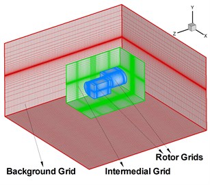
a) Overset grid profile
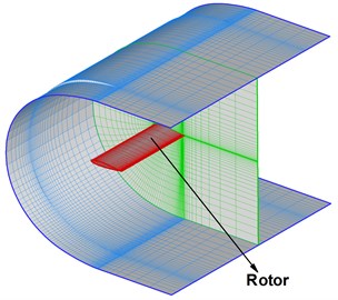
b) Rotor grid profile
3. Numerical methods
3.1. Governing equations
Under the assumption of continuous medium, three dimensional unsteady compressible Reynolds averaged Navier-Stokes (RANS) equations are given by the integral conservation form:
where:
with:
and , , , and are density, pressure, temperature, shear stress and heat conductivity coefficient. , , denote three Cartesian velocity components of fluid velocity . and express total energy and total enthalpy, and their relation is given by the formula . , , are three unit vectors along three coordinate axes of rectangular coordinate system, and with unit normal vector is the boundary of the control volume .
Eqs. (1) are not only suitable for static control volume, but also for arbitrary motion state. However, it is expected that the time derivative can be gotten out of the integral formula so as to conveniently solve equations with the finite volume method. According to the Leibniz theorem [24], there is the formula:
where is the boundary velocity vector of control volume. In other words, is mesh velocity vector. If Eq. (2) are plugged into Eq. (1), we can get the RANS equations with the integral form:
with:
To simulate the flow field of aircraft flight in the wind disturbance environment, it is supposed that perturbation of wind has the temporal synchronization in the computational domain considering the small size of the aircraft and the small wind perturbation, so the field velocity method is adopted. The flow fields can be construed as obtaining an equal and opposite velocity according to the relative motion. Based on the physical principle of the above building mathematical model, the convective terms of the RANS equations should be changed to:
Correspondingly, the governing equations are converted to:
and is the speed vector relative to the atmospheric disturbance. In the paper, the grid velocity for the wind disturbance is only carried out in the two regions of rotor grids. The information is transferred between the rotor grids and intermedial grid, as well as the intermedial grid and background grid via artificial external boundaries and hole boundaries, which embodies the advantage of moving overset girds.
The state equations are needed to guarantee the closure of control equations, which are written by:
where is the ratio of specific heats. The eddy viscosity is modeled by the zeroth-order algebraic turbulence model provided by Baldwin Lomax [25].
3.2. Conversion of coordinate system
Since the rotary wing motion is broken down by using three levels of overset grids, coordinate transformation is required to carry out among sub domain grids including intermedial grid, background grid and rotor grids during designing program of the unsteady flow field. Three kinds of coordinate systems are involved. One of the related coordinate systems is inertial coordinate system also called absolute coordinate system written as . Rotational coordinate system is obtained after the inertial coordinate rotates () around the axis, and rotor coordinate system is obtained after the rotational coordinate rotates around the axis. Here is azimuthal angle.
To define:
where is called transformation matrix from coordinate 2 to coordinate 1. Since all of the coordinate systems are orthogonal, the transformation matrices are all orthogonal matrices, that is to say:
Two basic transformation matrices are given by:
where, Coordinate transformation between overset sub domain grids is implemented by combining the above two basic matrices.
3.3. Discrete method
By using the finite volume method for Eq. (6) on each control volume , ordinary differential equations are obtained as the form:
with , , , , , .
For spatial discretization, second-order central differencing scheme is used to solve the viscous fluxes. Roe Riemann solver as a flux difference splitting scheme is adopted to approximate the inviscid fluxes. At the volume interface (), Roe scheme is given by the expression [26]:
where the subscript (, ) stands for the left and right physical variables across the interface (). denotes the Roe’s average matrix. It is worth noting that the eigenvalues of the Roe average matrix are:
where , , and . Entropy fix is required to avoid non-physical solution. We adopt Harten’s entropy fix [27].
To improve accuracy, fifth-order WENO-Z reconstruction [28, 29] is performed for the left and right physical variables in the Roe Riemann solver. In the curvilinear coordinate system with uniform distribution grids, interpolation is conducted dimension by dimension. Left state extrapolated primary variable of fifth order accuracy is expressed by:
where ( 0, 1, 2) is obtained by extrapolating cell average values in the stencil :
By nonlinear WENO-Z weight, can be written as:
where 0.3, 0.6, 0.1. The expression of smooth factor is given by literature [30]. The introduction of is to avoid the denominator becoming 0. Traditional choice is . However, if is too large relative to the computational grid, the solution containing discontinuity could be affected. It is proposed that is taken as a function of [29, 31], for example . We choose 10-18 because the smallest grid magnitude near body surface is 10-6. Right state value can be derived in a similar way on the stencil , 1, 2, 3.
The implicit scheme of dual time stepping is used for the time update [21]. One rotation period is divided into 1200 equal physical time stations. The computation of flow fields are iterated 5 steps at every physical time station, which is called pseudo time computational process. Main iteration and sub iteration correspond to the physical time process and the pseudo time process, respectively. The both processes are implicit, so the time update method is called implicit dual time step method.
Specially, to introduce pseudo time term in Eq. (11):
where is pseudo time, and is physical time. The physical time derivative is approximated by second-order backward difference of three points, and then we can get implicit discrete equations:
where:
stands for sub iterative residual. Therefore, the solutions of governing equations equal to the steady solutions of Eqs. (18) by updating pseudo time .
First order implicit backward difference is performed for the pseudo time derivative of Eq. (18):
where . With linearization for the inviscid flux , it can be derived as following:
with:
The sub iteration is solved by the use of implicit LU-SGS method [32]:
3.4. Initial conditions and boundary conditions
In order to accelerate convergence, pseudo steady is computed until density residual reaches four magnitude or iteration is carried out 1000 steps. The results are regarded as the initial fields.
Boundary conditions consist of body surface boundary condition for the rotary wings, slotted boundary condition for the C-H topological rotor grids, far field boundary condition for the outmost of the background grid, artificial external boundary and hole boundary conditions for transferring information between the rotor grids and intermedial grid, as well as the intermedial grid and background grid. It is a difficulty for the implementation of artificial external boundaries and hole boundaries when using high order schemes. The variables and of fifth order WENO scheme use the stencil including cell , , , , , thus we propose to adopt three layers of cell fingers of hole boundaries and artificial external boundaries so as to the direct implementation of interpolation without reducing order. The information exchange between overset grids is carried out by trilinear interpolation method.
4. Results and discussion
4.1. Flow field simulations without wind perturbation
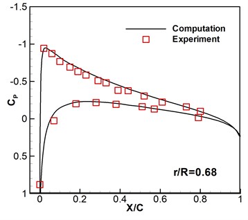
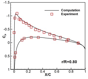
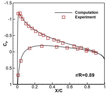
Caradonna-Tung two-bladed rotor [20] is selected to be the rotary-wing model. The rotary wings have two same blades which are made up of NACA 0012 sections and have a rectangular planform which has an aspect ratio of 6. To verify the codes and the computational overset grids, subsonic flows around hovering rotor are computed based on the available experimental data. The flight states are a pitch angle 8°, a tip Mach number 0.439, and a Reynolds number 1.98×10⁶. As shown in Fig. 2, the computed surface pressure coefficients are compared with the experimental data at the 0.68, 0.80, 0.89 and 0.96 spanwise stations. It can be seen that the numerical results are consistent with the experimental data. Then this solver is further developed to compute the flows of micro rotary wings under low Reynolds number with wind perturbation.
Fig. 2Computed and experimental surface pressure coefficient without wind disturbance

4.2. Aerodynamic response of micro rotary wings under wind disturbance
Computation is carried out for the flight conditions of pitch angle 6°, tip Mach number , and tip Reynolds number 1×10⁵. As shown in Fig. 3, since the most sensitive influence of atmospheric disturbance comes from that of perpendicular to the direction of incoming flow, we study small perturbation with sinusoidal wind that is parallel to the axial direction of the rotary wings.
The function of atmospheric perturbation in axial direction is expressed by:
Then the grid velocity function for the atmospheric disturbance is:
The blade tip velocity can be written as:
where is angular velocity and is radius rotation.
Fig. 3The sketch of rotary wings suffering disturbance of wind
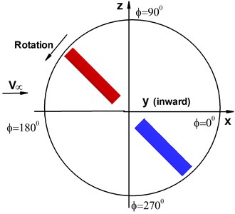
a) Rotational motion of rotary wings
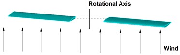
b) Atmospheric disturbance
Let , . To define ratio of perturbation amplitude and ratio of perturbation frequency:
the grid velocity function can be written as:
In the paper, the aerodynamic response of the micro rotary wings is studied at different disturbance frequencies with same disturbance amplitude, as well as different disturbance amplitudes with same disturbance frequency. Given the basic ratio of perturbation amplitude , the computational cases are expressed as follows: 0.5, 1.0, 2.0, as ; , , , as 1.0.
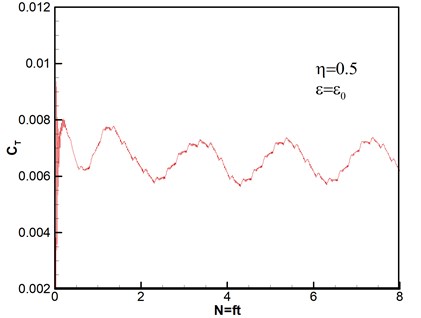
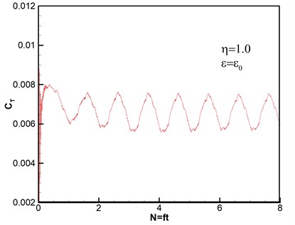
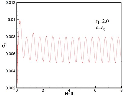
Thrust response under different disturbance frequencies is shown in Fig. 4. We can see that curves of thrust coefficient change with the number of rotary period under different disturbance frequencies based on the same amplitude , except that Fig. 4(a) is the case without wind disturbance. The number of rotation can be given by . And the expression of thrust coefficient is , where is the total thrust obtained by integral of pressure on the rotor blades [33]. Therefore, both of and are nondimensional parameters. It can be seen that all of thrust coefficients tend to stability after second rotational period, which reveals that the computational method has high good robustness. The flows are unsteady despite no disturbance as shown in Fig. 4(a). The varying frequencies of thrust agree with the wave frequencies of disturbance wind, however, the varying amplitudes gradually become stronger with the increasing of disturbance frequencies.
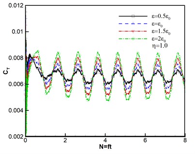
When the ratio of perturbation frequency , thrust response under different disturbance amplitudes of velocity is shown in Fig. 5. The thrust amplitude increases as disturbance amplitude of velocity increasing. Meanwhile, the varying frequencies of thrust are almost identical. The results are in accord with the actual conditions.
From the computational results, it can be predicted that the influence of wind perturbation could be controlled by adjusting the rotary wing pitch according to the changing frequency and amplitude of wind speed. Maybe, delay effect should be considered so as to nonlinear control algorithm would be adopted through combining CFD technique.
Fig. 4Thrust response under different disturbance frequencies
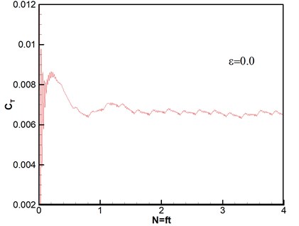
a)
b)
c)
d)
Fig. 5Thrust response under different disturbance amplitudes of velocity
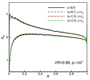
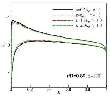
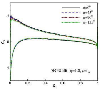
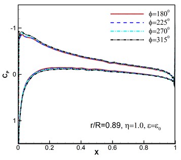
Furthermore, the computed surface pressure coefficients are illustrated at the spanwise station 0.89 in Fig. 6. Whether the pressure response results of different wind disturbance with the azimuthal angle 180° shown in Fig. 6(a)-(b) or different azimuthal angles with the same wind perturbation of , 1.0 shown in Fig. 6(c)-(d) are consistent with the flight situation. And the results conform to the flight aerodynamic characteristics.
Fig. 6Surface pressure coefficients under wind disturbance
a)
b)
c)
d)
5. Conclusions
One high fidelity numerical method is extended to compute the unsteady aerodynamic loads when rotary wings suffer sinusoidal wind. Field velocity method is effectively developed to the mathematics modeling for small wind perturbation in the condition of using moving overset grids. The grid velocity representing the wind perturbation is carried out in the rotor grids, and the flow information is transferred among overset grids by artificial external boundaries and hole boundaries, where three layers of fingers are proposed so that the fifth order WENO-Roe spatial discrete method is directly implemented for inviscid term instead of reduced order.
In the paper, the aerodynamic response of the micro rotary wings is researched at different disturbance frequencies and different disturbance amplitudes. The results show that atmospheric disturbance has an important impact on the flows of micro rotary wings under low Reynolds number. Thrust coefficient response presents periodic fluctuation and its amplitude is proportional to that of wind disturbance. The varying frequencies of thrust accord with the wave frequencies of disturbance wind, however, the varying amplitudes gradually become bigger with the increasing of disturbance frequencies. Most of all, it can be predicted from the results that the influence of wind perturbation could be controlled by changing the rotary wing pitch.
References
-
Lysak P. D., Capone D. E., Jonson M. L. Prediction of high frequency gust response with airfoil thickness effects. Journal of Fluids and Structures, Vol. 39, 2013, p. 258-274.
-
Han D., Wang H. W., Gao Z. Aeroelastic analysis of a shipboard helicopter rotor with ship motions during engagement and disengagement operations. Aerospace Science and Technology, Vol. 16, Issue 1, 2012, p. 1-9.
-
Wang L., Dai Y., Yang C. Gust response analysis for helicopter rotors in the hover and forward flights. Shock and Vibration, 2017, https://doi.org/10.1155/2017/8986217.
-
Dessi D., Mastroddi F. A nonlinear analysis of stability and gust response of aeroelastic systems. Journal of Fluids and Structures, Vol. 24, 2008, p. 436-445.
-
Zeiler T. A. Matched filter concept and maximum gust loads. Journal of Aircraft, Vol. 34, Issue 1, 2015, p. 101-108.
-
Drouot A., Richard E., Boutaye M. Hierarchical back stepping-based control of a gun launched mav in crosswinds: theory and experiment. Control Engineering Practice, Vol. 25, 2014, p. 16-25.
-
Raveh D. CFD-based models of aerodynamic gust response. Journal of Aircraft, Vol. 44, Issue 3, 2007, p. 888-897.
-
Parameswaran V., Baeder J. D. Indicial aerodynamics in compressible flow-direct computational fluid dynamic calculations. Journal of Aircraft, Vol. 34, Issue 1, 1997, p. 131-133.
-
Singh R., Baeder J. D. Direct calculation of three-dimensional indicial lift response using Computational Fluid Dynamics. Journal of Aircraft, Vol. 34, Issue 4, 1997, p. 465-471.
-
Zaide A., Raveh D. Numerical simulation and reduced-order modeling of airfoil gust response. AIAA Journal, Vol. 44, Issue 8, 2006, p. 1826-1834.
-
Bartels R. Development, Verification and Use of Gust Modeling in the NASA Computational Fluid Dynamics Code FUN3D. Technical Report, NASA/TM-2012-217771, 2012.
-
Bartels R. Developing an accurate CFD based gust model for the truss braced wing aircraft. 31st AIAA Applied Aerodynamics Conference, San Diego, United State, 2013.
-
Steijl R., Barakos G. N. Computational study of helicopter rotor-fuselage aerodynamic interactions. AIAA Journal, Vol. 47, Issue 9, 2009, p. 2143-2157.
-
Pahlke K., Van Der Wall B. Chimera simulations of multibladed rotors in high-speed forward flight with weak fluid-structure-coupling. Aerospace Science and Technology, Vol. 9, Issue 5, 2005, p. 379-389.
-
Dietz M., Kramer E., Wagner S. Tip vortex conservation on a main rotor in slow descent flight using vortex-adapted chimera grids. 24th AIAA Applied Aerodynamics Conference, Fluid Dynamics and Co-located Conferences, 2006.
-
Chen C., Prasad J. V. R. Simplified rotor inflow model for descent flight. Journal of Aircraft, Vol. 44, Issue 3, 2007, p. 936-944.
-
Webster R. S., Chen J. P., David L. Numerical simulation of a helicopter rotor in hover and forward flight. 33rd Aerospace Sciences Meeting and Exhibit, Aerospace Sciences Meetings, 1995.
-
Allen C. B. Parallel universal approach to mesh motion and application to rotors in forward flight. International Journal for Numerical Methods in Engineering, Vol. 69, Issue 10, 2007, p. 2126-2149.
-
Long L., Haisong A., Xun G. Design and numerical analysis of a novel coaxial rotorcraft UAV. Journal of Vibroengineering, Vol. 14, Issue 2, 2012, p. 1252-1262.
-
Caradonna F. X., Tung C. Experimental and Analytical Studies of a Model Helicopter Rotor in Hover. NASA Technical Memorandum 81 232, 1981.
-
Xu L., Weng P. F. High order accurate and low dissipation method for unsteady compressible viscous flow computation on helicopter rotor in forward flight. Journal of Computational Physic, Vol. 258, Issue 1, 2014, p. 470-488.
-
Chiu I. T., Meakin R. L. On automating domain connectivity for overset grids. 33rd Aerospace Sciences Meeting and Exhibit, Aerospace Sciences Meetings, 1995.
-
Meakin R. L. A new method for establishing intergrid communication among systems of overset grids. 10th Computational Fluid Dynamics Conference, Fluid Dynamics and Co-located Conferences, 1991.
-
Kundu P. K., Cohen I. M. Fluid Mechanics. Elsevier Academic Press, 2004.
-
Baldwin B. S., Lomax H. Thin layer approximation and algebraic model for separated turbulent flow. 16th Aerospace Sciences Meeting, Aerospace Sciences Meetings, 1978.
-
Roe P. L. Approximate riemann solvers, parameter vectors, and difference schemes. Journal of Computational Physics, Vol. 43, Issue 2, 1981, p. 357-372.
-
Harten A. High resolution schemes for hyperbolic conservation laws. Journal of Computational Physics, Vol. 49, Issue 3, 1983, p. 357-393.
-
Borges R., Carmona M., Costa B., Don W. S. An improved weighted essentially non-oscillatory scheme for hyperbolic conservation laws. Journal of Computational Physics, Vol. 227, Issue 6, 2008, p. 3191-3211.
-
Don W. S., Borges R. Accuracy of the weighted essentially non-oscillatory conservative finite difference schemes. Journal of Computational Physics, Vol. 250, 2013, p. 347-372.
-
Jiang G. S., Shu C. W. Efficient implementation of weighted ENO schemes. Journal of Computational Physics, Vol. 126, Issue 1, 1996, p. 202-228.
-
Henrick A. K., Aslam T. D., Powers J. M. Mapped weighted essentially non-oscillatory schemes: achieving optimal order near critical points. Journal of Computational Physics, Vol. 207, Issue 2, 2005, p. 542-567.
-
Yoon S., Jameson A. Lower-upper symmetric-gauss-seidel method for the Euler and Navier-stokes equations. AIAA Journal, Vol. 26, Issue 9, 1988, p. 1025-1026.
-
Johnson W. Helicopter Design. Princeton University Press, 1980.
About this article

This work was supported by the National Natural Science Foundation of China (No. 11502141, No. 11502139).
