A method for describing large rotations with a combination of axial and transverse Euler vectors

1. Introduction

In the problems of rotor dynamics of machines, which consist of shafts, gears, bearings and other rotating elements, in most cases the rotation along one of the directions (axial) is much greater than the rotations of the other two directions (transverse).

To describe the large rotations in geometry, physics and mechanics, a dozen methods are used [1-3]. The disadvantage of all methods of describing large rotations using 3 kinematic parameters (Euler angles, Cardan angles, rotation vectors) is the presence of singular points. The problem is that matrices or tensors connecting angular velocities with derivatives of kinematic parameters become degenerate when a certain critical value is reached by rotation.

The purpose of this article is to develop a different method for describing large rotations, taking into account the specific problems of the rotor dynamics of machines consisting of shafts, gears, bearings and other rotating elements. The main idea is to divide the general rotation of some assembly (shaft section, bearing ring, gear, etc.) into a rotation around the rotor axis and a transverse rotation. In most cases, for the listed rotating parts, the transverse rotation is limited by some not very large values. For example, even for spherical bearings, the relative transverse rotation of the rings cannot reach the value of $\pi$/2.

2. Description of large rotations using the Euler vector

The most effective and simple way to describe large rotations in the opinion of the authors is to describe it with the help of the Euler vector [4-8]. The vector description of the rotations is based on Euler’s theorem that an arbitrary combination of spatial rotations is equivalent to one plane rotation. The Euler vector just sets this plane rotation. Its direction indicates the axis of rotation, and the length is equal to the angle of rotation (Fig. 1).

Fig. 1Euler vector

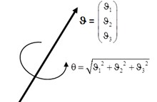
The following tensor functions of the vector argument are connected with the Euler vector:

where $\mathbf{\vartheta }$ – Euler vector; $\theta$ – the length of the Euler vector (Fig. 1); $\mathbf{L}\left(\mathbf{\vartheta }\right)$ – the function that calculates the rotation tensor with respect to a given Euler vector; $\mathbf{B}\left(\mathbf{\vartheta }\right)$ – the function that computes the tensor Zhilin by a given Euler vector; $\mathbf{E}$ – the unit tensor; $\mathbf{\vartheta }\mathbf{\vartheta }$ – the dyad product of the vectors $\mathbf{\vartheta }$; $\mathbf{\vartheta }$×$\mathbf{E}$ – a skew-symmetric tensor with a concomitant vector $\mathbf{\vartheta }$.

3. Description of large rotations with a combination of axial and transverse Euler vectors

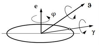
As shown in the introduction, the specific features of the rotor dynamics of machines consisting of shafts, gears, bearings and other rotating elements are the limitation of the transverse rotation. In this connection, it is not necessary to use the Euler vector for a total rotation, since the norm of this vector is limited to 2$\pi$, and thousands of rotations must be described. The vector of Euler is enough to describe the transverse rotation. Then, for the rotation around a fixed longitudinal axis, the usual rules of kinematics of plane motion from theoretical mechanics will operate. Therefore, it is convenient to represent the total rotation with the Euler vector $\mathbf{\vartheta }$ as a combination of two successive rotations – the first rotation around the axis of the rotor $\mathbf{e}$ by an angle $\phi$, the second rotation around an axis perpendicular to the axis of the rotor with the Euler vector $\mathbf{\gamma }$ (Fig. 2).

Fig. 2A combination of axial and transverse Euler vectors

In the case of small rotations, the separation of the total rotation into parts is achieved by projecting onto the rotor axis and onto the plane perpendicular to the axis. In the case of large rotations, it is necessary to involve the rotation tensors:

The rotation tensors differentiate according to the following formulas:

where $t$ – time; $\mathbf{\omega }$ – the total angular velocity; ${\mathbf{\omega }}_{\phi }$ – the angular velocity from rotation around the axis of the rotor; ${\mathbf{\omega }}_{\gamma }$ – the angular velocity associated with the change of the Euler vector $\mathbf{\gamma }$.

From Eqs. (1) and (2), as shown in [4], when two successive rotations are imposed, the rule of combining angular velocities follows:

Thus, the total rotation in fact can be determined accurately by using the separated Euler vectors $\phi \mathbf{e}$ and $\mathbf{\gamma }$: the first rotation around the fixed unit vector $\mathbf{e}$ by the angle $\phi$, the second around the transverse axis passing through the vector $\mathbf{\gamma }$ by the angle $\left|\gamma \right|$.

Since the first rotation is a plane rotation, the elementary formula of the kinematics of plane motion is valid for it:

For the second rotation, according to (1), the angular velocity is found using the Zhilin tensor:

Substituting (3) into (5) with regard to (4) allows us to express the derivative of the Euler vector $\mathbf{\gamma }$ using angular velocities:

Projecting the relation (6) to the axis of the rotor, taking into the orthogonality condition for the vectors $\mathbf{e}$ and $\gamma$, leads to the identity:

From (7) the expression ${\mathbf{\omega }}_{\phi }$ in terms of the total angular velocity shows:

Expressions (4) and (6), with supplementary Eq. (8), are the required differential equations of kinematics of rotational motion represented by the composition of two rotations $\phi \mathbf{e}$ and $\mathbf{\gamma }$.

4. The numerical example

As an example, let us consider the dynamics problem for a rotor fixed in a block of springs. The schematic diagram is shown in Fig. 3.

Fig. 3The position of the rotor at the initial time

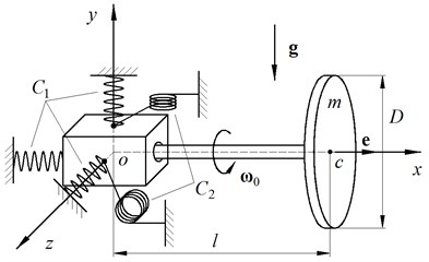
The spring assembly consists of 3 tension-compression springs with stiffness $C_1$ and 2 torsional springs with stiffness $C_2$. The rotor is a thin disk with mass $m$ and a weightless absolutely rigid rod with length $l$. At the initial time, when the rotor was positioned horizontally, it is given the initial angular velocity ${\mathbf{\omega }}_0$ around the axis of the rotor.

The numerical calculation was carried out for the following initial data:

• Disc diameter $D=$ 0.5 m;

• Rotor mass $m=$ 5 kg;

• The distance from the mass-center to the center of the block of springs $l=$ 0.75 m;

• Acceleration of gravity $g=$ 9.81 m/s²;

• Coefficients of spring stiffness $C_1=$ 2000 N/m and $C_2=$ 500 Nm/rad;

• Initial angular velocity ${\omega }_0=$ 50 rad/s.

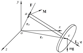
Fig. 4 shows the forces and moments acting on the rotor in the process of motion. The block of springs creates a force $\mathbf{F}$ at point $a$, directed opposite to the radius vector of point $a$, and a moment $\mathbf{M}$ directed opposite to vector $\mathbf{\gamma }$. In addition to the reactions of the springs, the gravity force $m\mathbf{g}$, applied at the center of gravity of the disk (point $c$), acts on the rotor.

Fig. 4The forces and moments acting on the rotor during the motion

The dynamics of the rotor is described by the following system of differential equations:

where ${\mathbf{r}}_c$ – the radius vector of the mass-center; ${\mathbf{v}}_c$ – the velocity vector of the mass-center; ${\mathbf{K}}_c$ – the vector of the angular momentum; ${\mathbf{r}}_a$ – the radius vector of the left end of the rotor.

When the system (9) was compiled, the kinematic relations (4), (6), (8) were used. The remaining equations are obtained from the usual equations of kinematics and rigid body dynamics.

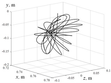
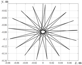
For numerical integration, the traditional fourth-order Runge-Kutta method with automatic step selection was used. The results of the calculation in form of trajectory of mass center are shown in Fig. 5.

Except for the motion of the mass-center of the rotor, we are also interested in the change of the axial angular velocity ${\omega }_{\phi }$, which in the problems of rotor dynamics is usually assumed to be constant. The deviation of ${\omega }_{\phi }$ from the initial angular velocity ${\omega }_0$ is shown in Fig. 6.

From Fig. 6 it shows that the axial angular velocity varies with time, but the deviation is very small (the greatest relative deviation $\left|{\omega }_{\phi }-{\omega }_0\right|/{\omega }_0$ does not exceed 0.1 %).

The result of the dynamics problem is checked by observing the law of conservation of total energy. The dependence of the combinations of energies on time is shown in Fig. 7.

Fig. 5The trajectory of mass-center

a)

b)

Fig. 6Deviation of the axial angular velocity from the initial angular velocity

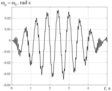
Fig. 7The dependence of the combinations of energies on time: 1 – Changes in kinetic energy; 2 – Changes in total energy; 3 – Changes in potential energy

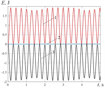
The total energy is stored with high accuracy. This accuracy confirms not only the absence of errors in the presented equations, but also the absence of numerical problems when using the proposed method of dividing the rotation into axial and transverse.

5. Conclusions

A kinematically accurate way of dividing a large rotation into an axial rotation and a transverse rotation is demonstrated, which has no singular points and allows considering infinitely large rotations, provided that the transverse rotation does not exceed 2$\pi$. The numerical example of a rotor fixed in a block of springs shows the absence of numerical problems when using the proposed method.

References

-
Branets V. N., Shmyglevsky I. P. Introduction to the Theory of Freeform Inertial Navigation Systems. Nauka, Moscow, 1992.
Bremer H. Elastic Multibody Dynamics: a Direct Ritz Approach. Springer, 2008.
Zhuravlev V. F. Fundamentals of Theoretical Mechanics. Second Edition, Publishing House of Physical and Mathematical Literature, Moscow, 2001.
Zhilin P. A. Vectors and Second-Rank Tensors in Three-Dimensional Space. Publishing House SPbSTU, St. Petersburg, 1992.
Zhilin P. A. Rational Mechanics of Continuous Media: Textbook. Publishing house of Polytechnic University, St. Petersburg, 2012.
Rankin C. C., Brogan F. A. An element independent corotational procedure for the treatment of large rotation. Journal of Pressure Vessel Technology-Transactions, Vol. 108, Issue 2, 1986, p. 165-174.
Crisfield M. A. Nonlinear Finite Element Analysis of Solid and Structures. John Wiley and Sons, Chichester, 1996.
Eliseev V. V., Zinovieva Т. V. Mechanics of Thin-Walled Structures. Theory of Rods. Publishing house SPbSTU, St. Petersburg, 2008.
About this article