Fault diagnosis method for rolling bearings based on the interval support vector domain description

1. Introduction

Rolling bearing is one of the most widely used devices in rotating machinery equipment. Its defects and damage will directly affect the performance and life of the whole mechanical equipment. Therefore, fault classification of the rolling bearing is of great practical significance to the normal operation of mechanical equipment. Under the engineering background, the contact gap will inevitably change when the machine works. This often leads to uncertainty in structural parameters. Therefore, the uncertainty of fault samples should not be ignored. Technically speaking, it is difficult for traditional fault diagnosis methods to have any effective impact on the above situation, because these methods only aim at deterministic fault samples. In recent years, uncertainty interval data classification is a research hotspot. Many scholars have made some representative research achievements in this field. Based on probability density, Sutar etc. put forward an interval data classification in the method of a boundary splitting [1]. This paper extends classical decision tree algorithms to handle data with interval values. Li etc. propose an interval data decision tree classification algorithm which is combined with evidence theory [2]. Aggawal provides a survey of interval data mining and management applications [3]. Naive Bayes, as a widely used classification method for deterministic samples, has aroused a lot of interest among relevant researchers. Qin etc. create the native Bayes uncertain classification method 1(NBU1) and the native Bayes uncertain classification method 2 (NBU2) [4]. NBU1 and NBU2 both use the parameter estimation method based on Gauss distribution assumption to calculate the class conditional probability density function of interval data. There is a slight difference between the two methods in the processing of the interval data model. However, NBU1 and NBU2 need the accuracy type of the class conditional probability density function of uncertain data. The formula-based Bayes classifier (FBC) algorithm, proposed by Ren etc., assumes uncertain interval data to meet the Gauss distribution [5]. The nonparametric estimation in the Parzen window method is applied to calculate the type of the class conditional probability density function of interval samples. However, as a kind of learning method, FBC needs all training samples to predict each rolling bearing fault repeatedly. Therefore, both the computational complexity and the memory requirements of this method are too enormous to be offered in fault diagnosis fields.

Support vector domain description (SVDD) is constructed based on the structured risk minimization theory [6-10]. The structured risk minimization, which is applied in this method, enables SVDD to generalize better in the unseen interval testing samples than neural networks etc. which apply empirical risk minimization. To make full use of these advantages and solve the fault diagnosis problem of rolling bearing interval data, this paper proposes an ISVDD through applying the Euclidean norm of two interval numbers as the distance in tradition SVDD. Because rolling bearing fault diagnosis application is a multi-class classification problem, ISVDD can reach multiple fault classification based on the posterior probability distribution function. In ISVDD model, there are two parameters: one is the penalty parameter which makes a trade-off between maximum margin and classification error, the other one is the radial basis function kernel width parameter. Both of the two parameters are chosen to improve the classification effect. Thus, the dynamic decreasing inertia weight particle swarm optimization (PSO) is utilized to select the optimal parameters [11].

This paper is organized as follows: Section 2 proposes the ISVDD method. Section 3 uses the dynamic decreasing inertia weight PSO to select the parameters for the ISVDD method. Section 4 analyzes the classification results of University of California Irvine (UCI) data. Section 5 applies ISVDD in rolling bearing faults diagnosis, as well as the comparison results with other methods. Finally, the conclusion is presented in Section 6.

2. The proposed ISVDD

The basic idea of the traditional SVDD is that a nonlinear function $\phi \left({\mathbf{x}}_i\right)$ maps ${\mathbf{x}}_i$ into a higher dimensional feature space and finds the smallest sphere that contains most of the mapped data points [9, 10]. This sphere can separate into several components when it is mapped back to the data space. Each component encloses a separate cluster of points. But, the traditional SVDD only aims at deterministic fault samples. Compared with the traditional SVDD, the proposed ISVDD aims at uncertainty interval fault samples. ISVDD is established on the theory of the traditional SVDD and the Euclidean norm of two interval numbers.

To construct ISVDD, there are also some preliminaries:

1) Given training data $\left\{\right({\mathbf{x}}_1,y_1),\dots ,({\mathbf{x}}_n,y_n\left)\right\}$. ${\mathbf{x}}_i$ is an interval data ${\mathbf{x}}_i=[{\underset{\_}{\mathbf{x}}}_i,{\overline{\mathbf{x}}}_i]$, $\phi \left({\mathbf{x}}_i\right)$ is a nonlinear function which maps ${\mathbf{x}}_i$ in to a higher dimension feature space.

2) In the ISVDD, the distance between training data ${\mathbf{x}}_i$ and the center of ISVDD is selected as the interval Euclidean norm [12]:

Now, the objective function of ISVDD is presented as follows:

where ${\xi }_i$ is the slack variable, $R$ is the radius of the minimum sphere, $\alpha$ is the center of the minimum sphere, $c$ is the penalty parameter. Compared with the traditional SVDD, the inequality constraint is replaced by the Euclidean norm of interval data in the proposed ISVDD. This optimization problem, including the constraints, can be resolved by solving the following Wolfe dual problem as follows:

where the RBF kernel $K({\mathbf{x}}_i,{\mathbf{x}}_j)=\phi \left({\mathbf{x}}_i\right)\cdot \phi \left({\mathbf{x}}_j\right)=\mathrm{e}\mathrm{x}\mathrm{p}(-{‖{\mathbf{x}}_i-{\mathbf{x}}_j‖}^2/\text{2}{\delta }^2$ with width parameter $\delta$ is used. Only those points with $\text{0}<{\beta }_j<C$ lie on the boundary of the sphere and are named support vectors. The trained Gaussian kernel support function, defined by the squared radial distance of the image of $\mathbf{x}$ from the sphere center, is then given by:

Since rolling bearing fault diagnosis application is a multi-class classification problem, ISVDD can reach multiple fault classification based on the posterior probability distribution function. The detailed procedure of the proposed method is as follows:

Step 1: Training data can be first divided into c-disjoint subsets according to their output classes. For example, the $i$th class dataset contains $N_k$ elements as $\left\{\right(x_{i1},{\omega }_k),\dots ,\{x_{i{N}_k},{\omega }_k\left)\right\}$.

Step 2: After solving the dual problem Eq.(8), ${\stackrel{-}{\beta }}_{il}$, $l=$1, …, $N_k$ and $J_k\subset \text{1},\dots ,N_k$ can be worked out as the set of the index of the non-zero ${\stackrel{-}{\beta }}_{il}$.The trained Gaussian kernel support function for each class data set $f_k\left(\mathbf{x}\right)$ is then given by Eq. (4).

Step 3: For each class data set, $k=\text{1},\dots ,c$, a posterior probability distribution function is estimated as $\delta \left({\omega }_k\right|\mathbf{x})=\left(f_k\left(\mathbf{x}\right)\right)/r_k$, where $r_k=R^2\left({\mathbf{x}}_{sk}\right)$ is the radius of the $k$th class sample sphere. $\left(f_k\left(\mathbf{x}\right)\right)/r_k$ is the relative distance which is adapted to identify the class type of the test object $\mathbf{x}$. the following rules can be gained as the following:

(1) Given a test object $a$, if $\left(f_a\left(\mathbf{x}\right)\right)/r_1\mathrm{}<\text{1}$ and $\left(f_a\left(\mathbf{x}\right)\right)/r_2\mathrm{}>\text{1}$, then $a$ belongs to the 1st class.

(2) Given a test object $b$, if $\left(f_b\left(\mathbf{x}\right)\right)/r_1>\text{1}$ and $\left(f_b\left(\mathbf{x}\right)\right)/r_2>\text{1}$, then $b$ belongs to the new class.

(3) Given a test object $c\text{,}$ if $\left(f_c\left(\mathbf{x}\right)\right)/r_1<\text{1}$ and $\left(f_c\left(\mathbf{x}\right)\right)/r_2<\text{1,}$ then $c$ belongs to $\mathrm{m}\mathrm{i}\mathrm{n}\{\left(f_c\left(\mathbf{x}\right)\right)/r_1\mathrm{},\left(f_c\left(\mathbf{x}\right)\right)/r_2\}$.

According to these rules, $\mathbf{x}$ can be classified as $\mathrm{a}\mathrm{r}\mathrm{g}\underset{k=1,\dots ,c}{\mathrm{m}\mathrm{i}\mathrm{n}}\delta \left({\omega }_k\right|\mathbf{x}).$

3. ISVDD model based on the dynamic decreasing inertia weight PSO

The dynamic decreasing inertia weight PSO [11]. As mentioned by Shi and Eberhart, is an improved algorithm based on the traditional PSO. It has many advantages, especially its excellent global optimization ability, simple operation and easy implementation, no selection, crossover, mutation and so on. In order to further improve the global optimization ability. Shi and Eberhart do not set the inertia weight as the fixed value, but set it to a function that decreases linearly with time, and the function of the inertia weight is:

${\omega }_{\mathrm{m}\mathrm{a}\mathrm{x}}=$ 1.2, ${\omega }_{\mathrm{m}\mathrm{i}\mathrm{n}}=$ 0.8. As mentioned by Shi and Eberhart, when the inertia weight is moderate ($\text{0.8}<\omega <\text{1.2}$), the dynamic decreasing inertia weight PSO will not only have the best chance to find the global optimum but also takes a moderate number of iterations through many experiments. On the contrary, when the inertia weight is low ($\omega \le \text{0.8}$), the search time is very short, that is, all the particles tend to gather together quickly. it will not find the global optimum. On the contrary, when the inertia weight is large ($\omega \ge \text{1.2}$), the algorithm always explores new regions. Of course, the algorithm needs more iteration to reach the global optimal. For these advantages, the dynamic decreasing inertia weight PSO is proposed to select the penalty parameter and the RBF kernel parameter of ISVDD model. This paper also draws a flowchart of the dynamic decreasing inertia weight PSO for ISVDD model in Fig. 1. In this method, the penalty parameter and the RBF kernel parameter are defined as the value of particles. The ISVDD classification accuracy is selected as the fitness function. Through the moving process forward and obtaining the optimal classification accuracy, particles will find the most significant the penalty parameter and the RBF kernel parameter for ISVDD.

Fig. 1Flowchart of the dynamic decreasing inertia weight PSO for ISVD model

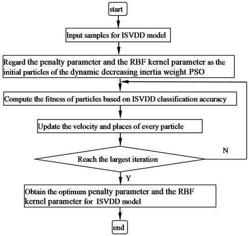
The detailed algorithm of the dynamic decreasing inertia weight PSO can be summarized as follows:

Step 1: Initialize the particles randomly so that each particle has the initial velocity $v_i^k$, $i=1,\dots ,n_{sw}$ and the initial position $x_i^k$, $i=\text{1},\dots ,n_{sw}$.

Step 2: Set the test function as the fitness value of the particles, calculates the fitness value of the initial particles according to the test function, and finds the individual extreme value $pbes{t}_{id}^k$ and the group extreme value $gbes{t}_{id}^k$.

Step 3: Compare each particle with its fitness $f_{id}^k$ and individual extreme $pbes{t}_{id}^k$. If $f_{id}^k>pbes{t}_{id}^k$, $pbes{t}_{id}^k$ is replaced by $f_{id}^k$.

Step 4: Update the particle position and velocity under the dynamic decreasing inertia weight, and checks whether the updated position $x_{id}^{k+1}$ and velocity $v_{id}^{k+1}$ cross the boundary:

Step 5: Runs at the preset maximum number of iterations, the algorithm stops and outputs the global optimal solution. Otherwise, return to Step 2 to continue the search.

4. The classification experiment of UCI data

In this experiment, the sample needs to introduce uncertain information into the deterministic dataset, because there is no open standard set of uncertain data. The standard data set used in the experiment is selected from UCI database [14]. The method of adding interval uncertain information is to add the uncertain information to each attribute $x_{ij}$ of any sample. The detailed method is the same as reference [15]. The interval samples of iris are obtained as in Table 1.

Now, the disposed of samples are used to train ISVDD to get the interval classification. In order to improve the classification accuracy of ISVDD, the penalty parameter $c$ and the RBF kernel width parameter $\delta$ are chosen by the dynamic decreasing inertia weight PSO algorithm. Generally, the bigger the penalty parameter is, the stronger the non-linear fitting ability is. However, if the penalty factor $c$is too large, serious over-fitting problems will occur, and the generalization ability of ISVDD will be reduced. In addition, the RBF kernel width parameter affects the kernel mapping distribution of data samples. Usually, the smaller the kernel parameter is, the better the nonlinear fitting performance of SVM is, and the stronger the noise sensitivity is. However, when the kernel parameters are set too small, the smoothing effect will be too small to affect the accuracy of the test set. Two sets of data (iris and wine) from the UCI database are used to estimate the sensitivities of the key parameters ($c$, $\delta$) on the classification results. Iris data set has 3 types and 4 attributes for each feature vectors. 30 samples are used as training samples. 90 samples are used as testing samples. Wine dataset has 3 types and 12 attributes for each feature vectors. 24 samples are used as training samples. 154 samples is used as testing samples. The dynamic decreasing inertia weight PSO are as follows:

Step 1: Initialize the parameter values of the algorithm as follows:

(1) Number of particles: $n=$ 50.

(2) The largest iteration number: $ite{r}_{\mathrm{m}\mathrm{a}\mathrm{x}}=$ 100.

(3) Inertia weight of PSO: ${\omega }_{\mathrm{m}\mathrm{a}\mathrm{x}}=$ 1.2, ${\omega }_{\mathrm{m}\mathrm{i}\mathrm{n}}=$ 0.8.

(4) Positive acceleration constants: $c_1=$ 1.4962, $c_2=$ 1.4962.

Step 2: The penalty parameter and RBF kernel parameter are used as particles of dynamic decreasing inertia weight PSO, and the particles are initialized by position $x_{id}^{}$ and velocity $v_{id}^{}$.

Step 3: Calculate the fitness of each particle. In ISVDD, classification accuracy is set as the fitness function.

Step 4: Use the method introduced in Eq. (5) to dynamically adjust the inertia weight value.

Step 5: Determine whether the algorithm satisfies the termination condition. Otherwise, turn back to step 3.

For iris data sets, the penalty parameter and RBF kernel width parameter of ISVDD are selected (27.385, 0.2371) by the dynamic decreasing inertia weight PSO algorithm. For wine data sets, the optimal penalty parameters and RBF kernel parameters of ISVDD are selected (37.17, 0.6759). The detail classification results of ISVDD with different parameters ($c$, $\delta$) are listed in Table 2. The iris data sets achieve best accuracy 98.98 % with the optimal penalty parameters and RBF kernel parameters. The wine data sets achieve best accuracy 90.91 %. But when ($c$, $\delta$) is the unreasonable setting of (5,0.1) and (50,1), classification results of ISVDD are affected by these unreasonable setting. In other words, it is very important to select the proper combined parameters ($c$, $\delta$) by the dynamic decreasing inertia weight PSO algorithm.

To further illustrate the effect of the proposed ISVDD, the classification results of NBU1, NBU2, FBC are used to compared with ISVDD. The classification results are shown in Table 3. For Iris data set, the classification accuracy of ISVDD is 3.31 % higher than NBU1 and NBU2. Moreover, the classification accuracy of ISVDD is 2.22 % higher than FBC. For Wine data sets, the classification accuracy of ISVDD is 6.49 % higher than NBU1. The accuracy of the ISVDD is higher than that of NBU1, NBU2, and FBC because the proposed method is constructed based on the structured risk minimization theory. This theory pays attention to the empirical risk minimization and the model complexity minimization simultaneously. For this reason, the over fitting problem can be avoided, and the proposed method has higher generalization ability for testing samples. Furthermore, the dynamic decreasing inertia weight PSO can obtain the optimal penalty parameter and the RBF kernel parameter and improves the accuracy of ISVDD because of its excellent global optimization ability. Classification accuracy of NBU1 and NBU2 algorithm is the same, which is reasonable since the NBU1 and NBU2 are similar and these two methods are only different in the equation of average value and standard deviation. As a lazy learning method, FBC needs all training samples to predict each rolling bearing fault repeatedly. Therefore, the memory requirements of this method are too enormous to be offered in fault diagnosis fields.

5. Fault diagnosis experiment for the rolling bearing

In this paper, the rolling bearing fault data is used to verify the effect of the proposed ISVDD. Bearing state consists of four categories: normal, inner race fault, outer race fault, and ball fault. Status of fault damage bearings is single damage. Damage diameter is divided into 7 mils, 14 mils, 21 mils, and 28 mils. All the vibration data of rolling bearing analyzed in this paper comes from Case Western Reserve University (CWRU) bearing data center in Fig. 2 [16]. The transducer is used to collect speed and horsepower data. The dynamometer is controlled so that the desired torque load levels could be achieved. The test bearing supports the motor shaft at the drive end. Vibration data are collected by using a recorder at a sampling frequency of 12 kHz for different bearing conditions. Tests are carried out under the different loads varying from 0 hp to 3 hp with1 hp increments. The corresponding speed varies from 1797 rpm to 1730 rpm. The deep groove ball bearing 6205-2RS JEM SKF is used in the tests.

Fig. 2a) Motor drive fault test platform, b) schematic diagram of the tests platform

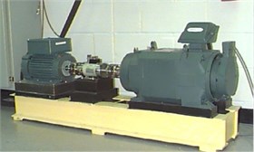
a)

b)

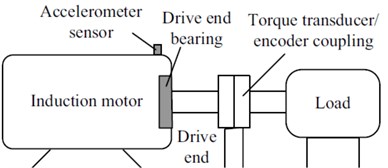
Various defect rolling bearings are produced by the electro-discharge machining in this test platform. Different rolling bearings, such as inner race fault, outer race fault, and ball fault are used to examine the proposed approach. Some defect rolling bearings are shown in Fig. 3

Fig. 3a) Outer race fault, b) inner race fault, c) ball fault

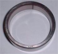
a)

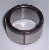
b)

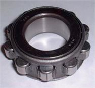
c)

Twelve fault types, such as normal bearing, inner race faults, outer race faults, and ball faults are used in this experiment. Some fault vibration signals are listed in Fig. 4.

Fig. 4Waveforms of rolling bearing fault vibration signals

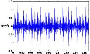
a) Inner race fault (7 mils)

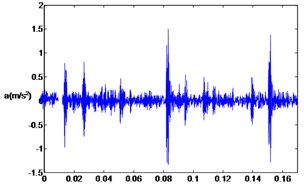
b) Inner race fault (14 mils)

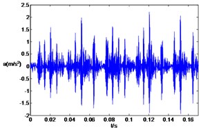
c) Inner race fault (28 mils)

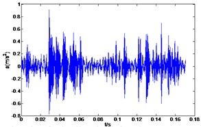
d) Ball fault (14 mils)

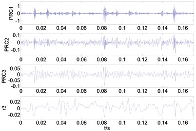
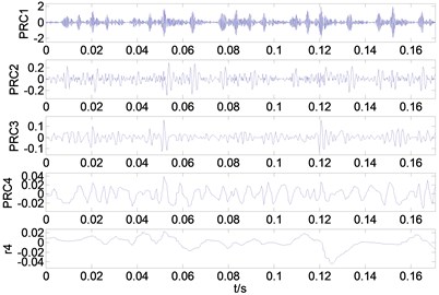
Now, intrinsic time scale decomposition (ITD) method is used to decompose the fault signal into several proper rotation components and a baseline component, which are decreased in frequency and amplitude [17-19]. The first few proper rotation components contain more shock signals. For these reasons, the instantaneous amplitude and instantaneous frequency sample entropy of the first three groups of proper rotation components are applied as the fault vibration signals feature vector. The specific operation steps are as follows:

1) After ITD decomposition of the signal, multiple proper rotation components (PR) and a baseline component are obtained. The decomposition results are given as Fig. 5.

2) Obtain the instantaneous amplitude, the instantaneous frequency of the 3 groups of PR.

3) Calculate the sample entropy of the instantaneous amplitude and instantaneous frequency. Each feature vector component is 6 dimensional because it includes the sample entropy of the instantaneous phase and instantaneous frequency of the first 3 group rotation components.

Fig. 5Decomposition results gained by ITD for four kinds of bearing vibration signals: a) the decomposition result of normal condition, b) The decomposition result of inner race fault (7 mils), c) the decomposition result of inner race fault (14 mils), d) the decomposition result of inner race fault (28 mils)

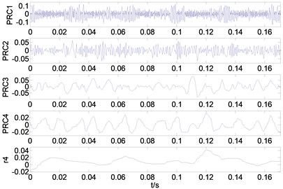
a)

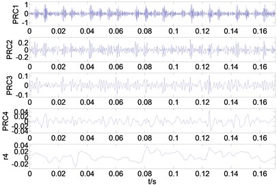
b)

c)

d)

By this means, then, 100 samples for each kind of fault signal can be obtained. Since there is no open, standard uncertainty rolling bearing fault number set, this experiment also introduces uncertainty information on the rolling bearing fault samples [13]. The detailed method for adding uncertainty information is the same as UCI on above.

Then, part of the training samples and testing samples are shown in Table 3. The amplitude entropy 1 in Table 4 represents the first rotation component instantaneous amplitude sample entropy, other characteristics and so on.

Now, the rolling bearing uncertain interval faults is used to compare the classification accuracy of NBU1, NBU2, FBC, and the proposed ISVDD method. In order to improve the accuracy of ISVDD, the penalty parameter and the RBF kernel parameter for ISVDD are chosen as (58.273, 0.8567) by the dynamic decreasing inertia weight PSO. The experimental results are shown in Table 5.

From Table 5, experimental results show that the classification accuracy of the proposed ISVDD is better than NBU1, NBU2 and FBC. According to Inner race fault (14 mils), the accuracy of ISVDD is 6.25 % higher than FBC, NBU1, and NBU2. Moreover, the total accuracy can be calculated：ISVDD: 96.46 %, FBC: 95.31 %, NBU1: 94.79 %, NBU2:94.58 %. The reason for such a high accuracy is the structural risk minimization principle and small sample properties in the learning process of ISVDD. moreover, the dynamic decreasing inertia weight PSO can obtain the optimal penalty parameter and the RBF kernel parameter and improves the accuracy of ISVDD.

6. Conclusions

This paper presents an interval fault classification method of the rolling bearing based on ISVDD. From the theory analysis and experimental results, it can be concluded that: (1) intrinsic time scale decomposition sample entropy is an effective feature index in fault identification for rolling bearing vibration signals. (2) After the hyper parameters of ISVDD are optimized by the dynamic decreasing inertia weight PSO algorithm, ISVDD method has the higher accuracy of the rolling bearing fault classification compared with the traditional interval fault classification methods. (3) The proposed method has been successfully applied to fault identification of the rolling bearing and the application demonstrates that the interval faults can be accurately and automatically identified. For the future work, we are trying to integrate the proposed method to process the rolling bearing compound faults under the uncertain structure parameters work condition.