Mathematical model of complex control of the vibratory transportation and technological process

1. Introduction

The vibratory transportation and technologic machines are widely used in various spheres of industry for transportation of friable materials and individual parts, measured feeding and sorting and also for carrying out various technologic operations on them [1-7].

The vibratory conveyors are especially effective for transportation of powdery, explosive, chemically aggressive, abrasive, heated and other friable materials, for the displacement of which, other types of conveyors are less suitable [1, 8].

The advantages of these machines are:

– Possibility of hermetization of the transportation and technologic processes that decrease the pollution of the environment;

– Elimination of losses and dirtying of the materials to be transported;

– Minimal wear of the working member;

– Compatibility of the process of transportation with scattering, heating, cooling, washing, mixing and other technologic operations.

In spite of the great number of researches in the sphere of the vibratory transportation and technologic machines, many unsolved problems remain in the direction of theory, design and fabrication. For example, the reasons of generation of the working member parasitic (non-working) vibrations [9] and their influence on the technologic process are studied insufficiently; such reasons may be incorrect transfer of the exciting force, features of the elastic system (springs) or other constructional errors (Fig. 1) [10].

In Fig. 1 is presented a two-mass system “vibro-drive – working member” and are shown spatial deviations of the working member caused by various possible errors: I – nominal (designed) position of the working member; II – position of the working member ($M_1$) considering the errors including the eccentricities $e_x$, $e_y$, $e_z$ of displacement of the center of gravity from position $O_1$ to point $O_1^{\text{'}}$; $O_2{O}_1^{\text{'}}$ – possible deviation of the exciting force; $\delta$ – possible deflection of the elastic element; ${\theta }_0$, ${\psi }_0$, ${\phi }_0$ – turnings of the coordinate axes caused by the assembly errors of the vibratory machine and transition from position $O_1{x}_1{y}_1{z}_1$ to position $O_1^{\text{'}}{x}_1^{\text{'}}{y}_1^{\text{'}}{z}_1^{\text{'}}$. 1 – basic elastic system of the vibro-machine; 2 – suspensions of the vibro-machine; $Q\left(t\right)$ – exciting force; the vibro-exciter ($M_2$ – $O_2{x}_2{y}_2{z}_2$) can also have the similar changes that are not shown in the drawing.

Fig. 1Deviations of the working member from the designed position stipulated by the vibro-machine design errors and spring specificity

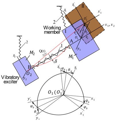
The axes $x_1$ and $x_2$ of the active and reactive parts ($M_1$and $M_2$) in this figure coincide in the initial position. The main interaction of the mentioned masses is realized along $x$ ($x_1$, $x_2$) axis that is reflected in the Eq. (7). The influence of vibrations of mass $M_2$on mass $M_1$ and respectively on mass $M_3$ in other directions is small in contrast to the influence of mass $M_1$on mass $M_3$, because in addition to elastic forces the interaction of inertial forces takes place here.

The aim of the work is to draw up the generalized mathematical model allowing to study the influence of the parameters and characteristics of masses of the system on the vibratory technologic process [11-16]. In this regard, it is expedient to consider spatial, relative-translatory and absolute movement of the three-mass dynamic system; it is analogous to the three-mass vibrational technological system, including the following parts: vibro-exciter, working member, load to be processed (to be transported).

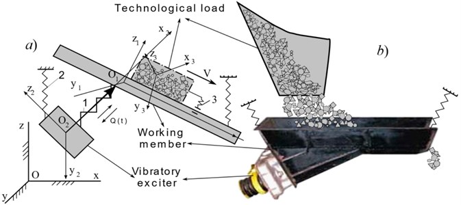
A dynamical model of the mentioned machine (Fig. 1(b)) is shown in Fig. 1(a), where to each mass the corresponding coordinate systems $O_1{x}_1{y}_1{z}_1$, $O_2{x}_2{y}_2{z}_2$, $O_3{x}_3{y}_3{z}_3$ are connected; $Oxyz$ – immobile (inertial) coordinate system; 1 – basic elastic system connecting a vibro-exciter to the working member, 2 – suspension of the vibratory machine, 3 – conventional elastic system connecting a friable load to the working member surface; $Q\left(t\right)$ – exciting vibratory force.

Though these masses are integrated into the common system, each of them is characterized by the proper physical and mechanical properties significantly different from each other; they should be taken into account at drawing up a generalized mathematical model of their movement.

For the inclusion of the technologic load (mass $M_3$) in the common spatial system (Fig. 4) and imparting it a generalized character, we present it as a rigid body connected to the WM ($M_1$) by the conventional elastic system 3 (Fig. 2), describing elastic and damping properties of the friable material.

At a fixed moment of time, elastic system 3 (as well as 1 and 2 in Fig. 2 and 3) is decomposed into three components, describing elastic properties of the material in space.

Fig. 2Vibratory technologic machine: a) generalized dynamical model; b) physical prototype with a bunker

A distinctive feature of the elastic system 3 is a non-retaining character of its connection with the WM in dynamics. With the help of the elastic-damping elements are described characteristics between the layers of the technologic friable materials, interaction between the layers and between the lower layer and WM. In contrast to the existing models [1, 2, 14, 16] all degrees of freedom are considered in it, i.e. it can be enclosed in the model of the general spatial system (Fig. 2, 3) and depending on the concrete problem, it can be reduced to the simpler form (plane, linear, null-dimensional).

Fig. 3A conventional elastic and damping system of the technologic load

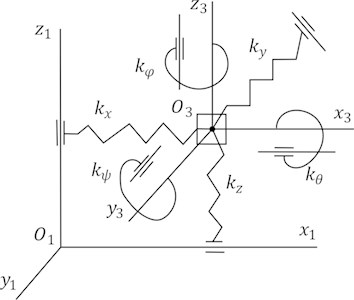
Presentation of the technologic load (TL) by the rigid body (at drawing up expressions of kinetic energy) is stipulated by the necessity of obtaining the equation of motion in the more generalized form not only for translational (in this case TL could be considered as a material point) but also for rotary movements.

The deformation of the friable TL layer is modeled at movement by the elastic elements with coefficients of elasticity $k_{x_3}$, $k_{y_3}$, $k_{z_3}$, $k_{{\theta }_3}$, $k_{{\psi }_3}$, $k_{{\phi }_3}$ (Fig. 3). The dissipation of energy at the deformation of the layer is considered by dampers with coefficients of resistance $C_{x_3}$, $C_{y_3}$, $C_{z_3}$, $C_{{\theta }_3}$, $C_{{\psi }_3}$, $C_{{\phi }_3}$ (not shown in Figure). Therefore, direct contact of the TL with WM is replaced by elastic-frictional connections.

2. Drawing up the mathematical model

For the deduction of the equations of movement, consider a spatial dynamical model of the system (Fig. 4).

The masses are considered in two positions (Fig. 4(b)): I – ideal-immobile, determined according to the design drawings, II – dynamical displacement under the action of the exciting force determined by the direction cosines in accordance with Tables 1 and 2, where $i=$ 1, 2, 3 (mass numbers), $m=$ I, II (positions of masses). Direction cosines in Table 2 are presented in the form of the angles of Euler-Krylov [17], where, because of small values of the rotary displacements, products of the angles no greater than second degree are taken into account at the expansion. Table 2 shows direction cosines for mass $M_1$(working member) only. For other masses, forms of expressions of the angles will be similar.

After dynamical displacement the positions of the coordinate systems will be: $O_1^{\mathrm{\text{'}}}{x}_1^{\mathrm{\text{'}}}{y}_1^{\mathrm{\text{'}}}{z}_1^{\mathrm{\text{'}}}$, $O_2^{\mathrm{\text{'}}}{x}_2^{\mathrm{\text{'}}}{y}_2^{\mathrm{\text{'}}}{z}_2^{\mathrm{\text{'}}}$, $O_3^{\mathrm{\text{'}}}{x}_3^{\mathrm{\text{'}}}{y}_3^{\mathrm{\text{'}}}{z}_3^{\mathrm{\text{'}}}$ (Fig. 4(b)).

Fig. 4A generalized model of the spatial movement of the vibratory technologic machine with a load

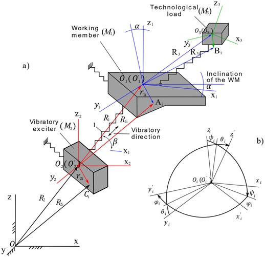
Fig. 4 shows the following indications: $A_i$, $B_i$, $C_i$ – free points of masses, $R_1$, $R_2$, $R_3$ – radius-vectors between the coordinate origin points (centers of masses), $R_{1i}^{\mathrm{\text{'}}}$, $R_{2i}^{\mathrm{\text{'}}}$, $R_{3i}^{\mathrm{\text{'}}}$ – $A_i$, $B_i$, $C_i$ – radius-vectors of the points relative to the origin of the coordinate axes of the corresponding masses, $r_{1i}^{\mathrm{\text{'}}}$, $r_{2i}^{\mathrm{\text{'}}}$, $r_{3i}^{\mathrm{\text{'}}}$ – $A_i$, $B_i$, $C_i$ – radius-vectors of the points relative to the origin of coordinate axes of own masses.

With the help of Fig. 2, 4 and methods of deduction of equations of motion of the material points and rigid bodies [5, 17], we obtain equations of spatial movement of masses $M_1$ and $M_3$.

The following ideas were taken into account in the establishment of the differential equations of motion:

– Spatial motion equations were established for the interconnected motion masses of the working body ($M_1$) and the technological load ($M_3$), as relative-translatory in relation to each other.

– Because $M_2$ is connected to mass $M_1$ by the potential and damping forces ($Q_q^{\mathrm{\text{'}}}$= $f\left(q_i,\stackrel{.}{q_i}\right)$, $i=$ 1, 2; $q=x_1,x_2,\dots ,{\phi }_2$) whose influence on the motion of the TL is insignificant, its spatial movement is described by linear differential Eq. (2); at the same time, $M_2$ as an electromagnetic vibro-drive realizes vibratory motion through angle $\beta$ with respect to mass $M_1$ (to the axis $O_1{x}_1$ of WM) by means of main elastic system 1 (Fig. 1 and 4).

– The influence of the mass of the load ($M_3$) on the working body ($M_1$) is indicated by coefficient $\mu$, the value of which could vary between 0-1 depending on a regime of the load movement (sporadic or with working body).

– In Eqs. (1) and (3), the multiplication type 2nd order nonlinear members will be considered mostly in the high amplitude (resonance) vibrations.

Working member motion equations will be as follows:

where ${\alpha }_1=\alpha +\beta$, $\alpha$ – the angle of inclination of the working member, $\beta$ – the angle of vibrations, $Q_{x_1}$, $Q_{y_1}$, $Q_{z_1}$ – components of the exciting force; $Q_{x_1}^{\text{'}}$, $Q_{y_1}^{\text{'}}$, $Q_{z_1}^{\text{'}}$ – elastic and damping forces from elastic systems 1 and 3 and weight of the TL; $A_{1\theta }$, $A_{2\theta }$, … – sum of the moments of inertia of masses relative corresponding axes, e.g.:

In the equation systems Eqs. (1) and (3), not all rotational movement equations are shown (in ${\psi }_1$, ${\varphi }_1$, ${\psi }_3$, ${\varphi }_3$ directions).

Spatial vibratory movements of mass $M_2$ are described by the equations:

where $C_{\theta }$, $C_{\psi }$, $C_{\varphi }$ are principal moments of inertia; $Q_{x_2}$, $Q_{y_2}$, $Q_{z_2}$ – components of the exciting force; $Q_{x_2}^{\text{'}}$, $Q_{y_2}^{\text{'}}$, $Q_{z_2}^{\text{'}}$ – elastic and damping forces from elastic systems 1 (they are functions of $q_{\mathrm{1,2}}$, ${\dot{q}}_{\mathrm{1,2}}$, where $q$ takes the values $x$, $y$, $z$, $\theta$, $\psi$, $\varphi$.

For technological load ($M_3$):

where $c_{x_1}$, $c_{y_1}$, $c_{z_1}$ – coefficients of resistance of WM elastic system; $B_{1\theta }$, $B_{2\theta }$, ... – functions of the sum of the inertia moments of masses relative corresponding axes; The coefficients $c_{x_1}$, $c_{y_1}$, $c_{z_1}$, $c_{x_3}$, $c_{y_3}$, $c_{z_3}$, $k_{y_3}$, $k_{z_3}$ (Fig. 3) in Eq. (3) change according to the movement of the material in relation to the working body ($z_3$) (the coefficient values reduce within the half period from the moment of detachment of the material from the surface [3, 5]).

The numerical values of stated (empirical) coefficients [3, 5] correspond to the ordinary coal with 5 % humidity, or ore with maximum fragment size no greater than 100 mm and with 2-3 % humidity.

For the description of the friction force between the WM and TL of the friable type various approaches [3, 18-20] are used, the essence of which is that reaction of the TL on WM is proportional to the velocity and deformation of TL (Fig. 3):

that will be written in the expanded form as follows:

where $q$ takes the values $x_3$, $y_3$, $z_3$; consequently, friction forces of the TL on the surfaces of WM (e.g. of the tray-shape form) and their moments will have the form:

where $f$ – coefficient of friction of the TL on the surface of WM; $r_q$ – distance between the friction surface and center of mass of the TL along the coordinate $q$.

Since the rotary movement of the material is relatively small than the linear one, and only the material’s longitudinal displacement is taken into consideration, only linear coordinates are provided for in the material friction forces Eqs. (5), (6).

Decomposing expression ${\left(F_{fr}\right)}_q$ along the surfaces of the WM, we obtain:

where $f_x$, $f_y$, $f_z$ – coefficients of friction along $x_1$, $y_1$, $z_1$; $N_y$, $N_z$ – normal reactions on the surfaces of the WM with tray-shape form; “$sign$” – non-linear function depending on sign of velocities ${\dot{x}}_3$, ${\dot{y}}_3$, ${\dot{z}}_3$: $sign$ = 1, at ${\dot{x}}_3{(\dot{y}}_3,{\dot{z}}_3)<0$; $sign$ = –1, at ${\dot{x}}_3{(\dot{y}}_3,{\dot{z}}_3)>0$. Moments of the friction forces will be determined by putting projections Eq. (6) into expressions of $M_q$ Eq. (5).

As it was mentioned, the TL (friable material) is unilaterally connected to WM (Fig. 3). It is periodically compressed and released depending on the action of the working member, or the pressure on the WM is increased and decreased (Fig. 2). The coefficients $c_{q_3}$ and $k_{q_3}$, change respectively in the expression $N_q=c_{q_3}{\dot{q}}_3+k_{q_3}{q}_3$ as well as in Eq. (3) in the process of modeling depending on $z_3$; When $z_3$ ≤ 0 (TL is displaced together with WM) values of $c_{q_3}$ and $k_{q_3}$ are significantly greater than when $z_3$ > 0 (TL loses contact partially or fully with WM) and these changes as well as the coefficients are different depending on the TL properties (dry, humid etc.) [3].

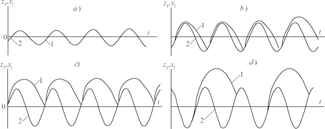
For illustration, in Fig. 5 is shown the trajectory of the friable material layer ($z_3$) relative to the working member vibration ($x_1$) [21].

Analysis of the oscillograms shows that the vibratory movement trajectory of the friable material layer, at various amplitudes of the working member vibration, is different: a) the material moves on the working surface with slipping without losing the contact with it; b) with increase of the amplitude the material loses the contact partially with the surface; c) with further increase of the amplitude a single touch of the material with the surface takes place during one period of the vibration followed by its jump (vibration velocity at losing the contact ${\dot{x}}_1=max$); d) with increase of the vibration amplitude (with increase of the velocity) the length of the material jump increases but since the vibration velocity is small at the moment of the material falling it cannot lose the contact until the velocity reaches the maximum again (the oscillogram of the vibration velocity ${\dot{x}}_1$ is not given in the Figure and it is meant that it is shifted from the displacement $x_1$ by the phase 90°).

The modeling was carried out according to the parameters of the resonant vibro-feeder with 500 W electro-magnetic vibro-exciter [5, 23-26]. At that, equations of movement of mass $M_2$ are replaced by the equation of variation of the electromagnetic flow $Ф$ [27]:

depending on which the exciting force is determined:

where $W$ – number of windings of the coil, $\delta$ – initial clearance between the magnet pole and anchor; ${\mu }_0$ – magnet penetration of the air; $S$ – area of the electromagnet core section; $r$ – total resistance; $x$ – displacement of the reduced mass of the active and reactive parts of the vibratory feeder.

The following assumptions were considered during the modeling:

– Movement of the material is presented at modeling by system Eq. (3) and reaction of the TL on WM is not provided for in Eq. (1) of the working member or $\mu$ = 0, which we often find in the researches [1-4, 7] and it does not change the qualitative characteristics of the results (in general, $\mu$ varies between 0-1 and its value depends on the type of friable material and vibration regime: that is the next stage of our research and the subject of our next publication).

– Only linear coordinates are provided for in the material friction forces Eqs. (5), (6), which is explained above.

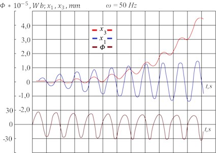
Fig. 6 shows some oscillograms of movement of the vibro-feeder with the load: vibrations of the working member – $x_1$, displacement of the friable material – $x_3$ and variation of the electromagnetic flow $\mathrm{Ф}$.

The mentioned oscillograms are obtained from the solutions of Eqs. (1), (3), (7) and (8) equations, when special non-working vibrations $y_1$, $z_1$, ${\theta }_1$, ${\psi }_1$, ${\varphi }_1$ are far from the working resonance (50 Hz).

Fig. 51 – trajectory of a grain movement (z3), 2 – amplitude of the working member (x1), a) displacement of a grain without losing touch with the working member, b), c), d) –displacement of a grain with losing touch with the working member

The process of the vibro-feeder’s entering the resonance, when amplitude $x_1\mathrm{}$of the working member and respectively angle of rise of the material displacement $x_3$ increase, is depicted in the picture; It should be noted in this connection that the equation of the material longitudinal displacement (first equation of (3)) does not include elastic deformation $x_3$ of the material (Fig. 3) because displacement of the material is not restricted in this direction (the working member groove is open in the longitudinal direction) in contrast to directions $y_3$ and $z_3$, when the working member bottom and walls restrict the material displacement and therefore, their equations include $y_3$ and $z_3$; Consequently, the material vibratory displacement $x_3$ has the form [3], shown in Fig. 6 and with increase of the velocity, angle of its rise increases.

Fig. 6Oscillograms of vibrations of the working member x1, variation of the electromagnetic flow Ф and displacements of the technologic load x3

In view of the fact that the exciting force in Eq. (1) presents in the non-linear form Eq. (8), there are two resonant positions at variation of the frequency – basic (50 Hz), sub-harmonic (25 Hz) and super-harmonic (100 Hz) that is reflected in the obtained results (Fig. 7, 8). The pictures show the dependence of the velocity of the longitudinal displacement of a friable material ($V_x$) on the variation of the rotary (${\psi }_1$), and vertical ($z_1$) vibration frequencies (${\omega }_{{\psi }_{\mathrm{}}}$ and ${\omega }_z$) of the working body ($M_1$), during their passage in resonance areas (25, 50, 100 Hz).

The influence of partial vibrations ($z_1\text{,}$${\psi }_1$ etc.) on the process (velocity) of material displacement is realized by means of the non-linear terms of Eq. (3), where they appear (e.g.$\mathrm{}{\ddot{\psi }}_1{z}_3$, ${\ddot{z}}_1{\psi }_1$ etc.).

The mathematical model was adjusted to reach the identicality with the physical experiment [3, 5, 15] to achieve the reliability of the modeling results: a vibratory displacement velocity of the friable material (ground coal) was measured on the real vibro-feeder. Then a simple numerical experiment was carried out by variation of the material model coefficients (Fig. 3) and were selected those values of the coefficients at which the results ($V_x$) of the physical and numerical experiments were identical.

At modeling the working member operates constantly in the basic (working) resonant mode (${\omega }_{exc}={\omega }_x=$ 50 Hz). Besides, the sub- and super-harmonic resonant vibrations with 25 (1/2 ${\omega }_{exc}$) and 100 Hz (2 ${\omega }_{exc}$) are also generated in the electromagnetic vibrator feeded from the 50 Hz (${\omega }_{exc}$) power supply network, by corresponding change of the rigidity. If we vary coefficients of rigidity i.e. eigenfrequencies ${\omega }_y$, ${\omega }_z$, ${\omega }_{\theta }$, ${\omega }_{\psi }$, ${\omega }_{\phi }$ in the equations of the working spatial vibrations in the range of 0-110 Hz, we obtain resonant vibrations of 25, 50, and 100 Hz in these directions. With such approach it becomes possible to enhance nonworking spatial vibrations and study their influence on the material velocity in combination with basic working resonant vibration (${\omega }_x=$ 50 Hz = const).

The graphs shown on Fig. 7 are obtained from the solutions of Eqs. (1), (3), (7) and (8), when the vibration of only $z_1$ direction enters into resonance and other non-working vibrations $y_1$, ${\theta }_1$, ${\psi }_1$, ${\phi }_1$ are far from the working resonance regime ($A=$ 2.8 mm, ${\omega }_x=$ 50 Hz), their influence is insignificant and the change of the longitudinal displacement velocity ($V_x$) depends on only non-working (“parasite”) change of $z_1$.

Fig. 7Dependence of the velocity of the longitudinal displacement Vx of the load M3 on the frequency of the WM resonant vibrations along axis O1z1; ωx= 50 Hz, A= 2.8 mm

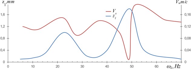
The graphs on Fig. 8 are also obtained from the solutions of Eqs. (1), (3), (7) and (8), when the vibration of only ${\psi }_1$ direction enters into the resonance, whereas the rest of non-working vibrations $y_1$, $z_1$, ${\theta }_1$, ${\phi }_1$ are far from the continuous working resonance regime ($A=$ 2 mm, ${\omega }_x=$ 50 Hz), i.e. they show the change of the longitudinal displacement velocity ($V_x$) depending only on the change of ${\psi }_1$. The change of $V_x$ on Fig. 7 and Fig. 8 begins when $z_1$ and ${\psi }_1$ non-working vibrations begin to enter the resonance and end when they exit the resonance, i.e. in the following limits of ${\omega }_z$ and ${\omega }_{\psi }$ frequencies 10 $>{\omega }_z>\mathrm{}$55 Hz, 35 $>{\omega }_{\psi }>$ 105 Hz. Outside of those frequencies, the value of $V_x$ is constant: on Fig. 7 $V_x\approx$ 0,12 m/s, on Fig. 8 $V_x\approx$ 0,08 m/s and they correspond to the nominal (experimental) values when the vibro-feeder mainly operates in the resonance regime and no outside factors affect the process of material displacement.

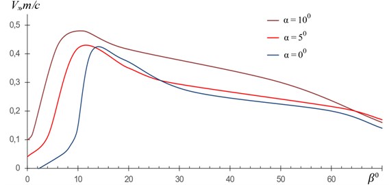
The graphs on Fig. 9 are obtained from the solutions of Eqs. (1), (3), (7) and (8), when all of the non-working vibrations $y_1$, $z_1$, ${\theta }_1$, ${\psi }_1$, ${\phi }_1$ are far from the working resonance regime ($A=$ 4 mm, ${\omega }_x=$ 50 Hz) and their influence on the process is insignificant; the graphs show the dependence of the friable material’s velocity on the angle of vibration ($\beta$) at fixed values of the angle of inclination of the working member ($\alpha$). As it is seen from the graph, the best result is reached at angles: $\alpha \approx$ 10° and $\beta \approx$ 10°.

Fig. 8Dependence of the velocity of the longitudinal displacement Vx of the load M3 on the frequency of the WM rotary vibrations ψ1; ωx= 50 Hz, A= 2 mm

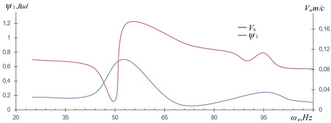
Fig. 9Dependence of velocity Vx of the friable material on the variation of the angle of vibrations β at fixed angles of the inclination of the working member α; ωx= 50 Hz, A= 4 mm

The working resonance frequency of the WM during the modeling process is constant: ${\omega }_x=$ 50 Hz = const.

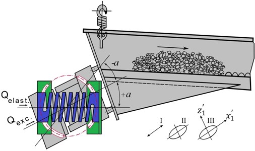
Fig. 10Design of the vibro-feeder with a controllable trajectory of vibrations of the working member

The results of the modeling have shown that some combinations of the spatial (non-working) vibrations and basic working vibrations may have a positive influence on the transportation and technologic process of the material (increase both, transportation velocity of the friable material and the intensity of movement).

Fig. 10 shows a design of the vibro-feeder with a new vibro-exciter. It is developed on the basis of the results of the modeling and it allows generation of various forms (I, II, III) of the working vibrations with the help of the variation of the angle between electromagnetic and elastic forces and thereby control the vibratory technologic process of the friable material.

3. Conclusions

1) A new mathematical model of spatial movement of the three-mass system – analog of the vibratory (Fig. 4) machine with technological load, is developed. A system of differential equations describes the interconnected movement of component parts of the loaded machine and allows many-sided research into vibratory transportation and the technologic process of the friable materials.

2) The presented graphs of the results show that mathematical modeling may reveal new nuances promoting improvement of both, the technologic process and the machine design.

3) It was, for example, ascertained that some spatial non-working (parasitic) vibrations in combination with basic (working) vibrations can significantly increase velocity of the material’s vibratory displacement (see Figs. 7, 8).

4) A new design of the electromagnetic vibratory feeder was developed on the base of the modeling results that allows obtaining various configurations of the working vibrations and increasing velocity of the material transportation by the change of the elastic force direction. The obtained design (Fig. 10) confirms reliability of the developed mathematical model because the influence of the vertical partial (non-working) vibration is qualitatively identical for both – the modeling (Fig. 7 – $z_1$) and the design (III-$z_1^{\mathrm{*}}$).