Tunnel surrounding rock stability prediction using improved KNN algorithm

Huang, Shuai; Qi, Qingjie; Liu, Jianzhong; Liu, Wengang

doi:10.21595/jve.2020.21427

Journal of Vibroengineering

Browse Journal

Submit article

Published: 15 November 2020

Check for updates

Tunnel surrounding rock stability prediction using improved KNN algorithm

Shuai Huang¹

Qingjie Qi²

Jianzhong Liu³

Wengang Liu⁴

¹Institute of Crustal Dynamics, China Earthquake Administration, Beijing, 100085, P. R. China

^{1, 2, 3, 4}China Coal Research Institute, Beijing, 100013, P. R. China

Corresponding Author:

Qingjie Qi

Cite the article Download PDF

Downloads 1211

WoS Core Citations 4

CrossRef Citations 6

Abstract

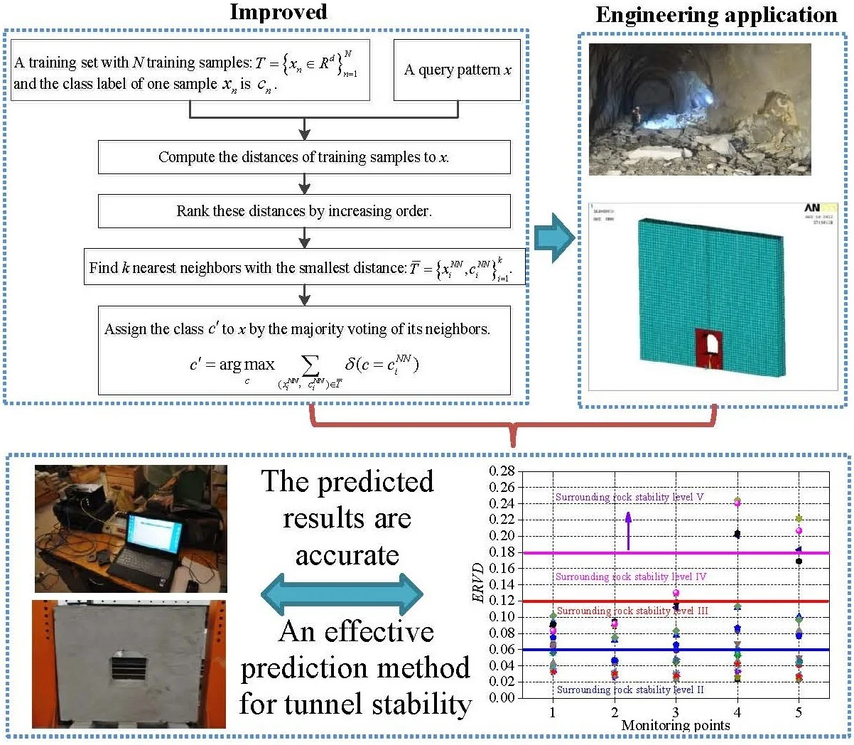
Accurate prediction of the stability of rock surrounding a tunnel is important in order to prevent from rock collapse or reduce the hazard to personnel and traffic caused by such incidents. In our study, a KNN algorithm based on grouped center vector is proposed, which reduces the complexity of calculation, thus improving the prediction performance of the algorithm. Then, the improved KNN algorithm was applied to the surrounding rock stability prediction of a high-speed railway tunnel, which, to our knowledge, forms the first application thereof for the prediction of surrounding rock stability. Extensive experimental results show that our proposed prediction model achieves high prediction performance in this regard. Finally, a laboratory experiment of a tunnel is conducted to evaluate whether the tunnel surrounding rock is stable or not. The experimental results matched the prediction results obtained by our proposed prediction model, which further demonstrates its effectiveness.

Tunnel surrounding rock stability prediction using improved KNN algorithm

Highlights

A KNN algorithm based on grouped center vector is proposed.
The improved KNN algorithm was applied to the surrounding rock stability prediction.
Our proposed prediction model can be used to assess the damage extent of the tunnel.
Our proposed prediction model achieves high prediction performance.

1. Introduction

The evaluation of surrounding rock stability is one of the key points in the construction project of highway and railway tunnels, mines and hydraulic power plants. Surrounding rock stability prediction is a method which applies the engineering analogism method to carry on surrounding rock stability evaluation, and it provides a basis for engineering design and construction, so it has important practical value. The prediction accuracy will directly affect the safety of engineering construction. The traditional prediction method is difficult to classify the of surrounding rocks stability quickly due to their depending on more geotechnical parameters [1, 2]. Consequently, the reasonable prediction method of surrounding rock stability should be of practical significance. The aim of this work is to obtain a prediction approach of the surrounding rock stability based on machine learning techniques.

Prediction of the surrounding rock stability is still a challenge, because there are so many factors, and they influence each other, moreover the surrounding rock stability has a complex nonlinear relationship with the influencing factors. Thus, it is difficult to predict the surrounding rock stability due to the various and complicated factors [3]. In the recent years, the machine learning theory, which has a very good modeling capability, has being developed unceasingly. The machine learning can carry on nonlinear operation, and has a strong self-learning ability and adaptive ability, so it is a good solution to nonlinear problems [4, 5]. Qiu et al. [6] established the prediction system of surrounding rock stability based on QGA (quantum genetic algorithm)-RBF (radical basis function) neural network and obtained a good evaluation result. Yuan et al. [7] chose five indexes including rock quality, rock uniaxial saturated compressive strength, structural surface intensity coefficient and amount of groundwater seepage as the model input, and established the prediction model for surrounding rock stability based on the support vector machine, and the results showed that the stability prediction results by GSM (grid search method)-SVM (support vector machine) model for surrounding rock corresponded to the actual results. Li et al. [8] analyzed the stability of surrounding rock of underground engineering by using an improved BP neural network, and the results showed that the leading roles of rock stability were rock mass quality, strength and state, and the structural plane occurrence and characters were secondary factors. Li et al. [9] established a prediction model for the surrounding rock stability based on PNN (probabilistic neural network), and the results showed that the PNN model had strong recognition ability and fast running speed and high calculation efficiency for the prediction of surrounding rock stability in a coal mine. Consequently, machine learning approaches are being increasingly used for estimating the surrounding rock stability.

It is worth noting that the k-nearest neighbor (KNN) algorithm [10-12], which is one of the most well-known algorithms in pattern recognition, has been proven to be very effective in prediction. The $k$ -nearest neighbor (KNN) algorithm, as one of the basic machine learning algorithms, is simple to learn and is widely used to solve prediction problems. The KNN algorithm is a new algorithm that evolves based on the idea of the nearest neighbor (NN) algorithm. The idea of a NN algorithm is to find the training samples which are nearest to the samples to be classified, and the category of the nearest training samples is used for category determination. The KNN algorithm contains the idea of the NN algorithm which is a special case where $k$ in the KNN algorithm is 1. The KNN algorithm does not need to estimate parameters and train the training set, and it is suitable for prediction with a large sample size. Furthermore, for solving a multi-label prediction problem, its performance is superior to that of the support vector machine (SVM) algorithm. As first proposed by Cover and Hart, it remains one of the most important machine learning algorithms until now, however, for the KNN algorithm, the similarity of each sample to be classified with all samples in the training set needs to be calculated. When there are too many training samples, it becomes time-consuming and therefore presents high calculation complexity, which is not conducive to rapid prediction. At present, there are two main aspects to improvements of the KNN algorithm: improving the accuracy and efficiency of prediction. To improve the prediction accuracy, scholars have carried out studies by adjusting its weights [13, 14]. Dudani [15] proposed a weighted voting method named the distance-weighted $k$ -nearest neighbor (WKNN) rule, which is the first distance-based vote weighting schemes. Gou et al.[16] presented a dual weighted k-nearest neighbor (DWKNN) rule that extended the linear mapping of Dudani, in which the closest and the farthest neighbors are weighted the same way as the linear mapping, but those between them are assigned smaller values. Furthermore, some new ideas are proposed to improve the selection of the $k$ value, and attempts are made to do so dynamically. The KNN algorithm generally requires a pre-set $k$ value and runs multiple experiments with different $k$ values to obtain the best prediction results. Moreover, the $k$ value selected at this time is used as the default experimental parameter. In view of this, Zheng [17] proposed a strategy of dynamically setting $k$ values. Liu et al. [18] propose a scheme reconstructing points of the test dataset by learning a correlation matrix, in which different $k$ values are assigned to different points of test data based on the training data. The KNN algorithm is widely used in pattern prediction, but some problems occur therewith. When calculating the similarity, the samples to be classified need to be compared with each sample in the training set by using the traditional algorithm, which depends on the number of training samples. If there are too few training samples, the prediction accuracy will be reduced.

On this basis, the KNN algorithm based on grouped center vectors is improved, and can group sample vectors under each category, and the center vectors in each group under this category can be used to represent the sample vectors in the training set under this category. This not only ensures the number of representative vectors and improves classification accuracy, but also reduces the number of training sets and improves the efficiency of the method when calculating the similarity values. Then our proposed prediction model is used for evaluation of surrounding rock stability of a high-speed railway tunnel. Finally, an indoor model experiment is conducted to see the prediction performance for surrounding rock stability of the high-speed railway tunnel including stability and instability. Extensive experimental results show that our proposed prediction model achieves much better prediction performance to the surrounding rock stability.

2. Our improved KNN algorithm

Before presenting our improved KNN algorithm, a brief review of KNN, WKNN and DWKNN algorithms is made.

2.1. KNN, WKNN and DWKNN

KNN, as a simple, effective, non-parametric prediction method, was first proposed by Cover and Hart to solve the text prediction problems [19]. Its principle is to expand the area from the test sample point $x$ constantly until $k$ training sample points are included. In addition, the test sample point $x$ is classified into the category which most frequently covers the nearest $k$ training sample points.

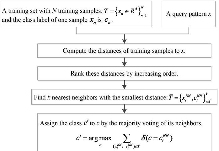
(1) The $k$ -nearest neighbor algorithm (KNN) [10] is a powerful nonparametric classifier which assigns an unclassified pattern to the class represented by a majority of its $k$ nearest neighbors. In the general classification problem, let $T = {\{x_{n} \in R^{d}\}}_{n = 1}^{N}$ denote a training set with $M$ classes including $N$ training samples in $d$ (dimensional feature space). The class label of one sample $x_{n}$ is $c_{n}$ . Given a query point $x$ , the rules to KNN algorithm are as follows. KNN algorithm implementation steps are shown in Fig. 1.

Fig. 1KNN algorithm implementation steps

(2) Dudani [15] first introduced a weighted voting method for KNN, calling the distance-weighted $k$ -nearest neighbor rule (WKNN). In WKNN, the closer neighbors are weighted more heavily than the farther ones, using the distance-weighted function. The weighted function of WKNN is shown in Eq. (1):

1

w_{i} = \{\begin{array}{l} \frac{d_{k} - d_{i}}{d_{k} - d_{1}}, d_{k} \neq d_{1}, \\ 1, d_{k} = d_{1}, \end{array}

d_{i} = \sqrt{(x - x_{i}^{N N})^{T} (x - x_{i}^{N N})},

where $d$ is the dimensional feature space; $k$ is the nearest neighbor; $x$ is the query point; $w$ is the weight.

Accordingly, the prediction result of the query is made by the majority weighted voting, as defined in Eq. (2):

2

c^{'} = a r g m a x \sum_{({x_{i}}^{N N}, {c_{i}}^{N N}) \in \bar{T}} δ, (c = {c_{i}}^{N N}),

where $c'$ is the classification result; $N$ is the training sample.

(3) DWKNN [16] is based on WKNN: Different weights are given to $k$ nearest neighbors according to their distances, with closer neighbors having greater weights. The dual distance-weighted function of DWKNN is defined in Eq. (3):

3

w_{i} = \{\begin{array}{l} \frac{d_{k} - d_{i}}{d_{k} - d_{1}} \cdot \frac{d_{k} + d_{1}}{d_{k} + d_{i}}, d_{k} \neq d_{1}, \\ 1, d_{k} = d_{1} . \end{array}

Then, the query $\bar{x}$ is labeled by the majority weighted vote of $k$ nearest neighbors, as specified in Eq. (4):

4

c' = \underset{c}{a r g m a x} \sum_{({x_{i}}^{N N}, {c_{i}}^{N N}) \in \bar{T}} w_{i} δ, (c = {c_{i}}^{N N}) .

2.2. Support vector machine (SVM) [20]

The main idea of SVM is summarized as follows: by giving a training sample set, a hyperplane established through SVM is used as a pattern surface, so that the space between the positive and negative examples of the two types of samples is maximized. The training samples on the hyperplane are known as support vectors. SVM is mainly used for analysis based on the linear separability. As for the pattern of linear inseparability, it is necessary to expand the basic idea of the algorithm. By introducing a kernel function, the linear inseparability in a low-dimensional space is transformed into linear separability in the high-dimensional space. Owing to the number of support vectors being much less than the number of training samples, a high prediction speed and accuracy can be obtained by using an SVM. From the perspective of linear separability, the SVM is required to find a decision function, as shown in Eq. (5):

5

f (x) = s g n (〈a \cdot x〉 + b),

where $〈a \cdot x〉$ represents the dot product of $a$ and $x$ , while $y = 〈a \cdot x〉 + b = 0$ is considered as the hyperplane.

The concepts of positive and negative examples are described as follows:

If $〈a \cdot x〉 + b \geq 0$ , it can be considered that $x$ is a positive example, that is $f (x) = 1$ .

If $〈a \cdot x〉 + b < 0$ , it can be regarded that $x$ is a negative example, namely $f (x) =$ –1.

Fig. 2 presents the geometric structure of the optimal hyperplane in the two-dimensional input space.

2.3. Our improved KNN algorithm

Different weights are to be allocated to $k$ nearest neighbors, and the weight $w_{j}$ of the $j$ -th nearest neighbor is determined as shown in Eq. (6):

6

w_{j} = \{\begin{array}{l} \exp (- ((\frac{d_{k} - d_{j}}{d_{k} - d_{1}}) ∙ (\frac{d_{k} + d_{1}}{d_{k} + d_{j}}))), & d_{k} \neq d_{1} . \\ 1, & d_{k} = d_{1} . \end{array}

The prediction model of the surrounding rock stability based on our improved KNN algorithm can be expressed as follows.

Let $X$ denote a set of surrounding rock stability sample, and suppose $X$ is $X = {\{x_{n} \in R^{m}\}}_{n = 1}^{N}$ , where $x_{i}$ represents the feature of the $i$ -th surrounding rock stability sample, N is the total number of features, and $m$ is the feature dimension. In addition, let $y_{i}$ represents the surrounding rock stability levels, and $y_{i} \in \{0,1, 2,3, 4\}$ , $i = 1,2, \cdot \cdot \cdot, N$ . Therefore, the sample set of the prediction model is shown in Eq. (7):

7

[\begin{matrix} x_{1} \\ x_{2} \\ \cdot \\ \cdot \\ \cdot \\ x_{N} \end{matrix} \begin{matrix} y_{1} \\ y_{2} \\ \cdot \\ \cdot \\ \cdot \\ y_{N} \end{matrix}] = [\begin{array}{l} {x_{1}}_{1} & {x_{1}}_{2} & \cdot & \cdot & \cdot & {x_{1}}_{m} & y_{1} \\ {x_{1}}_{1} & {x_{1}}_{2} & \cdot & \cdot & \cdot & {x_{2}}_{m} & y_{2} \\ \cdot & \cdot & \cdot & \cdot & \cdot & \cdot & \cdot \\ \cdot & \cdot & \cdot & \cdot & \cdot & \cdot & \cdot \\ \cdot & \cdot & \cdot & \cdot & \cdot & \cdot & \cdot \\ {x_{N}}_{1} & {x_{N}}_{2} & \cdot & \cdot & \cdot & {x_{N}}_{m} & y_{N} \end{array}] .

Given the unknown sample $x = (x_{1} x_{2} \cdot \cdot \cdot x_{m})$ , our proposed surrounding rock stability prediction model based on our improved KNN algorithm can be expressed as Eq. (8):

8

\bar{y} = \underset{w_{i}}{a r g m i n} f_{i} (x) = \underset{w_{i}}{a r g m i n} d (x, {\bar{x}}_{i}^{P N N}),

where ${\bar{x}}_{i}^{P N N}$ is the nearest neighbor of the unknown sample $x$ in the class $w_{i}$ ( $i = 1,2, 3$ ). Hence, the unknown sample $x$ is classified into the class $\bar{y}$ that has the closest neighbor among all classes.

3. Surrounding rock stability prediction based on our improved KNN algorithm

The prediction model is established using the training samples in reference [21]. There are 30 cases used for training and 23 cases are used for testing.

3.1. Influencing factors and surrounding rock stability prediction

The surrounding rock stability prediction is provided to find the nonlinear relationship between the influencing factors and the surrounding rock stability. The surrounding rock which is influenced by many factors is a highly nonlinear complex dynamic system. Therefore, the internal and external factors affecting the surrounding rocks stability shall be considered. In addition, it is impossible and not necessary to consider all of the influencing factors in the prediction model at present. So according to a large number of on-site observation results and practical experience, with reference to literature [22], the representative factors-rock quality designation (RQD, %), rock uniaxial saturated compressive strength ( $R_{w}$ , MPa), rock integrity coefficient ( $K_{v}$ ), structure plane strength coefficient ( $K_{f}$ ) and the amount of underwater seepage ( $W$ , L·min^-1) are chosen as the influencing factors.

According to China’s standard [22] and the domestic and international experience of surrounding rock stability prediction [23], surrounding rock stability is divided into 5 levels. The five levels are labeled as I, II, III, IV and V respectively, as depicted in Table 1.

Table 1Levels of surrounding rock stability prediction

No.	Levels	RQD (%)	$R_{w}$ (MPa)	$K_{v}$	$K_{f}$	$W$ (L·min^-1)
0	I	100-90	200-120	1.00-0.75	1.0-0.8	0-5
1	II	90-75	120-60	0.75-0.45	0.8-0.6	5-10
2	III	75-50	60-30	0.45-0.30	0.6-0.4	10-25
3	IV	50-25	30-15	0.30-0.20	0.4-0.2	25-125
4	V	25-0	15-0	0.20-0.00	0.2-0.0	125-300

3.2. Normalization

Since the range of each factor is significantly different, and the test results may rely on the values of a few factors, they are preprocessed using the normalization process [24]. The upper and lower margins of each factor and the process for the used normalization are computed as per Eq. (9), Eq. (10) and Eq. (11):

9

{\bar{y}}_{i} = \frac{y_{i} - y_{m i n}}{y_{m a x} - y_{m i n}},

10

y_{m i n} = m i n \{y\} = \underset{j = 1, \cdot \cdot \cdot \cdot \cdot \cdot, n}{m i n} \{y_{j}\},

11

y_{m a x} = m a x \{y\} = \underset{j = 1, \cdot \cdot \cdot \cdot \cdot \cdot, n}{m a x} \{y_{j}\},

where $y = (y_{1}, y_{2}, \cdot \cdot \cdot \cdot \cdot \cdot, y_{n})$ is each predictor.

Accordingly, the value of each factor is normalized to between 0 and 1 based on the Eq. (9), Eq. (10) and Eq. (11).

3.3. Criteria for our prediction approach performance

The accuracy, computed based on the percentage of all test samples classified correctly, is used to evaluate the prediction performance of the surrounding rock stability. Accuracy tells us about the number of samples which are correctly classified, and it is defined as follows:

12

A c c u r a c y = \frac{# t e s t s a m p l e s c l a s s i f i e d c o r r e c t l y}{# t e s t s a m p l e s},

where the $# t e s t s a m p l e s$ denotes the total number of test samples; the $# t e s t s a m p l e s c l a s s i f i e d c o r r e c t l y$ is the number of test samples that are classified correctly.

3.4. Prediction of surrounding rock stability

In this section, our proposed prediction model is pretested in 30 typical surrounding rock stability cases and tested in 23 typical surrounding rock stability cases. The neighborhood size $k$ ranges from 1 to 10 with an interval of 1, which is inspired by Ref. [24]. The 30 typical surrounding rock stability cases are shown in Table 2 and the 23 typical surrounding rock stability cases are shown in Table 3. This prediction experiment is implemented in eclipse 3.7.2 by Java language programming, and the hardware environment is Inter Core i7-6700 CPU 3.40 GHz.

As shown in Table 3, our proposed prediction model has high accuracy and reliability, and the prediction results of proposed prediction model are in good agreement with the actual results. The accuracy of our proposed prediction model is up to 91.30 %. This illustrates that our proposed prediction model is feasible to predict the surrounding rock stability, which shows that our proposed prediction model can be used to evaluate the stability of tunnel surrounding rock before the design and construction of the tunnel engineering.

Table 2Training samples of surrounding rock stability

No.	RQD	$R_{w}$ (MPa)	$K_{v}$	$K_{f}$	$W$ (L·min^-1)	Level
1	0.06	216.60	0.87	0.97	3.86	I
2	0.05	241.78	0.90	0.95	0.19	I
3	0.03	257.70	0.85	0.92	2.69	I
4	0.03	244.65	0.85	0.93	3.06	I
5	0.04	270.61	0.89	0.95	2.08	I
6	0.20	158.00	0.68	0.82	6.36	II
7	0.18	161.14	0.67	0.75	6.80	II
8	0.15	148.70	0.69	0.78	7.33	II
9	0.21	164.82	0.66	0.76	8.13	II
10	0.18	188.49	0.63	0.83	7.81	II
11	0.32	83.25	0.44	0.60	17.21	III
12	0.32	76.82	0.48	0.63	17.92	III
13	0.35	77.18	0.40	0.62	16.25	III
14	0.31	85.11	0.38	0.60	15.74	III
15	0.32	72.71	0.46	0.57	18.77	III
16	0.31	73.89	0.43	0.56	16.45	III
17	0.32	64.41	0.39	0.48	18.07	III
18	0.36	61.14	0.42	0.53	15.10	III
19	0.31	69.14	0.34	0.55	17.14	III
20	0.29	77.34	0.47	0.56	19.36	III
21	0.49	41.93	0.25	0.32	34.60	IV
22	0.51	36.48	0.28	0.27	71.27	IV
23	0.52	31.18	0.23	0.30	75.97	IV
24	0.57	37.54	0.22	0.28	67.92	IV
25	0.46	37.80	0.24	0.25	71.62	IV
26	0.84	8.77	0.07	0.12	157.42	V
27	0.76	13.06	0.08	0.15	200.26	V
28	0.84	11.92	0.11	0.31	159.93	V
29	0.73	7.65	0.08	0.75	173.72	V
30	0.81	17.43	0.06	0.11	184.46	V

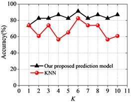
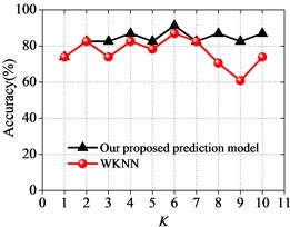
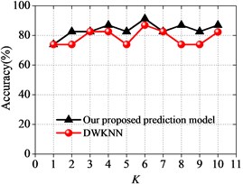
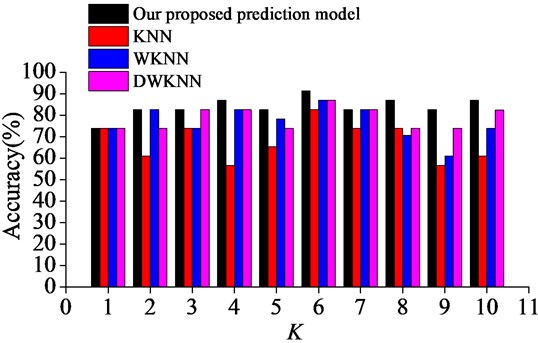
Next, the prediction performance of our proposed prediction model is compared with other prediction models based on KNN algorithm [11], WKNN algorithm [15], DWKNN algorithm [16] and SVM algorithm [24]. The following prediction experiments will show whether our proposed prediction model will achieve better prediction performance. The comparison results between different prediction models are shown in Fig. 2 and Fig. 3.

Fig. 2Prediction results for our proposed approach compared with other approaches

a) KNN algorithm

b) WKNN algorithm

c) DWKNN algorithm

As it can be seen in Fig. 2 and Fig. 3, the prediction accuracy of our proposed prediction model is somewhat better than the prediction accuracy of the prediction models based on KNN, WKNN and DWKNN algorithms in almost all of the test cases. It also shows that our proposed prediction approach performs better than other approaches with the increasing of the neighborhood size $k$ . It can be found that the accuracy of our proposed prediction model is the highest when the neighborhood size $k$ is 6, and our proposed prediction model achieves an accuracy of 91.30 %. This result suggests that our proposed prediction model based on the improved KNN algorithm has the robustness to the sensitivity of different choices of the neighborhood size $k$ with a good prediction performance in predicting the surrounding rock stability.

Table 3Test samples of surrounding rock stability

No.	RQD	$R_{w}$ (MPa)	$K_{v}$	$K_{f}$	$W$ (L·min^-1)	Level	Prediction results using our proposed model	Comment
1	0.26	36.0	0.22	0.35	5.0	IV	IV	Right
2	0.50	40.2	0.50	0.50	10.0	III	III	Right
3	0.52	25.0	0.20	0.50	5.0	III	III	Right
4	0.71	90.0	0.35	0.30	18.0	II	II	Right
5	0.24	12.5	0.13	0.18	125	V	V	Right
6	0.78	90.0	0.57	0.45	10.0	II	II	Right
7	0.50	70.0	0.50	0.25	5.0	III	II	Fault
8	0.42	25	0.22	0.35	12.5	IV	IV	Right
9	0.32	20.0	0.23	0.25	46.0	IV	IV	Right
10	0.51	26.0	0.26	0.35	20.0	III	III	Right
11	0.76	90.0	0.45	0.52	8.0	II	II	Right
12	0.22	13.5	0.10	0.15	135	V	V	Right
13	0.80	95.0	0.50	0.45	0.0	II	II	Right
14	0.35	70.5	0.35	0.30	10.0	III	III	Right
15	0.50	90.0	0.50	0.25	5.0	III	III	Right
16	0.05	93.0	0.60	0.50	0.0	II	II	Right
17	0.20	10	0.18	0.19	130	V	V	Right
18	0.30	70.0	0.40	0.20	10.0	III	IV	Fault
19	0.85	92.0	0.70	0.50	10.0	II	II	Right
20	0.40	25	0.28	0.35	35	IV	IV	Right
21	0.87	95.0	0.50	0.45	0.0	II	II	Right
22	0.41	20	0.25	0.3	30	IV	IV	Right
23	0.24	13.4	0.15	0.16	120	V	V	Right

Fig. 3Surrounding rock stability prediction results with different neighborhood sizes

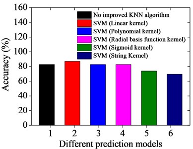
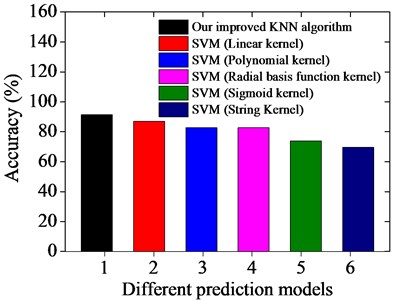
In addition, support vector machines algorithm is regarded as a simple and effective classification method based upon the statistical learning theory. Consequently, the experiments are also conducted to compare the prediction results based on the unimproved KNN algorithm and our improved KNN algorithm with the prediction result based on the SVM algorithm, as shown in Fig. 4. In this experiment, the neighborhood size $k$ is fixed as 6.

Fig. 4Prediction results based on different prediction models

a) Unimproved KNN algorithm

b) Improved KNN algorithm

As it can be seen in Fig. 4, the test samples are predicted by using the traditional KNN algorithm and our improved KNN algorithm when $k$ is fixed as 6, and the accuracy of our improved prediction model is maximized and obtains good prediction results. The accuracy of the prediction results based on the unimproved KNN algorithm and our improved KNN algorithm are 82.60 % and 91.30 %; while the accuracy of the prediction results based on the SVM with linear kernel, polynomial kernel, radial basis function kernel, sigmoid kernel and string Kernel are 86.95 %, 82.60 %, 82.60 %, 73.91 % and 69.56 %, respectively. Consequently, the results obtained using our improved KNN algorithm are stable, and the method offers higher prediction accuracy than the SVM algorithm.

4. Engineering application of our proposed prediction model

It is well known that the classification of surrounding rock stability can be realized by both theoretical method and finite element method; however, the two methods are complicated in engineering application, and the evaluation efficiency is low. Therefore, a prediction model based on improved KNN algorithm is proposed in the previous section. In this section, our proposed prediction model is used to predict the surrounding rock stability, and the predicted results are compared with the theoretical method and finite element method.

To determine the performance of our proposed prediction approach based on improved KNN algorithm in engineering applications, some experiments were also conducted to see the prediction performance for evaluating the tunnel surrounding rock stability along the high-speed railway from Jakarta to Bandung in Indonesia, and the prediction results were compared with the results computed by the finite element method. The reason for our study using the finite element method is that tunnel instability is an elastoplastic problem and complex nonlinear mechanics problem, and the mechanism of tunnel instability is rather complex, so suitable or convenient mechanics models are not available. Therefore, the analytical solution cannot be realized, while the finite element method can accurately simulate the tunnel instability process. The geological distribution of our research region is as shown in Fig. 5.

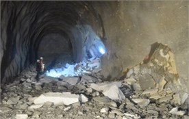
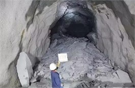
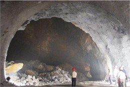
The tunnel engineering of our study is located in a legend along the high-speed railway from Jakarta to Bandung in Indonesia. Our research group participated in the seismic safety assessment of the high-speed railway from Jakarta to Bandung in Indonesia, and accumulated a large number of field survey data. The research region, dominated by mountainous regions, is mainly formed on the surface of an obduction plate due to the eruption of Cenozoic island arc volcanic rocks (basalt and andesite). Bangka and Belitung Islands are composed of Triassic intrusive rocks and Sedimentary rocks as the basement. Tunnels destruction cases along the railway are shown in Fig. 6.

Fig. 5Geological distribution of our research region

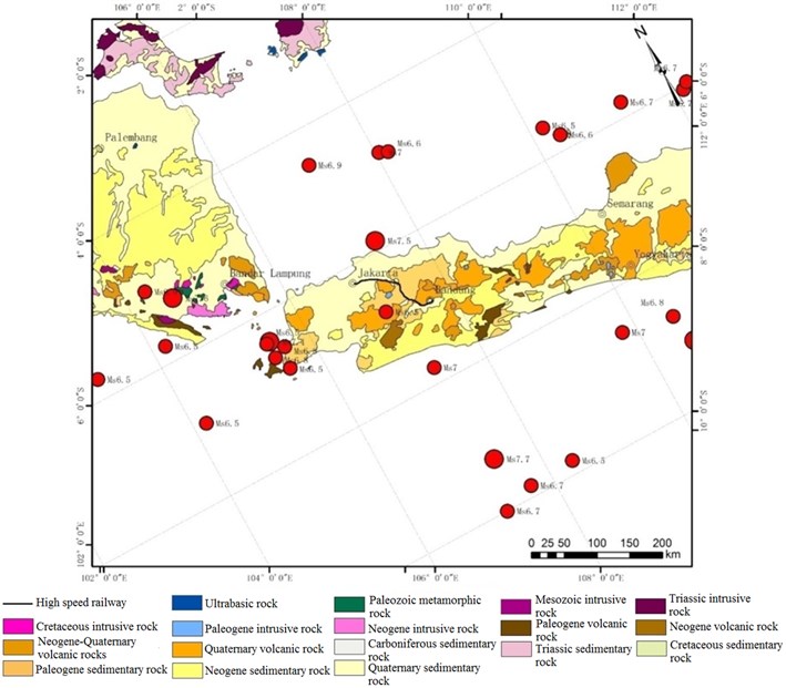
Fig. 6Tunnels destruction cases along railway

4.1. Finite element model of tunnel surrounding rock

In this section, the finite element model of the tunnel surrounding rock is established, and the surrounding rock stability levels are determined by changing the different influencing factors.

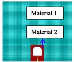
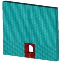
The tunnels along the high-speed railway from Jakarta to Bandung in Indonesia were chosen as the research object, and the finite element model was established. The finite element model of the tunnel surrounding rock is established using ANSYS software, as shown in Fig. 7. The model length is 150 m, the height is 130 m and the thickness is 12 m. The vertical distance is 32 m between the tunnel bottom and the model bottom. The tunnel length is 20 m and the height is 20 m. The element type is SOLID185, and the Mohr-Coulomb elasto-plastic model is used to simulate the stress-strain behavior of the rock. The model is divided into 13120 grid cells. Fixed constraint is applied at the bottom of the model. Meanwhile, in order to avoid the reflection of the model boundary to the stress wave, non-reflecting boundary conditions are applied to the top and sides of the model to simulate infinite boundaries.

Fig. 7Finite element model

The physical and mechanical parameters of the model materials are mainly obtained by on-site investigation and laboratory tests, as shown in Table 4. The surrounding rock stability cases along the high-speed railway are shown in Table 5.

Table 4Physical and mechanical model parameters

Type	Gravity density (kN/m³)	Internal friction angle (°)	Cohesion (MPa)	Elasticity modulus (GPa)	Poisson’s ratio	Tensile strength (MPa)
Material 1	23.8	37	0.6	2.6	0.327	3.02
Material 2	22.7	28	0.3	1.9	0.342	1.68

Table 5Surrounding rock stability cases along high-speed railway

No.	RQD	$R_{w}$ (MPa)	$K_{v}$	$K_{f}$	$W$ (L·min^-1)
1	0.52	25.0	0.22	0.52	12.0
2	0.41	25.0	0.22	0.35	12.5
3	0.28	26.0	0.32	0.30	18.0
4	0.41	20.0	0.25	0.30	30.0
5	0.76	132.0	0.78	1.85	3.5
6	0.20	10.0	0.18	0.19	130.0
7	0.80	100.0	0.58	1.70	8.0
8	0.22	13.5	0.10	0.15	135.0
9	0.51	45.0	0.35	0.50	5.0
10	0.50	40.5	0.38	0.55	10.5
11	0.24	16.5	0.15	0.15	125.0
12	0.91	132.0	0.83	0.85	5.5

4.2. Evaluation index of surrounding rock stability

The test signal changes when a fracture occurs inside the rock. The damage degree inside the rock can be determined by extracting the location of the mutation point in the signal and determining its singularity (or smoothness). In our study, energy ratio variation deviation (ERVD) is used to assess the surrounding rock stability levels. Wavelet energy spectrum can be constructed by transforming the frequency band energy ratio variation (ERV), and a quantitative correlation is available between wavelet energy spectrum and rock mass damage pattern. According to the change of frequency band energy ratio variation, the damage degree of the surrounding rock could be assessed as shown in Eq. (13):

13

E R V = \{E R V_{j}\} = \{|P_{c j} - P_{d j}|\}, j = 0,1, 2, \cdot \cdot \cdot \cdot \cdot \cdot, k - 1 .

where $E R V_{j}$ is the change of energy ratio in the $j$ frequency band of the wavelet frequency band energy spectrum; $P_{c j}$ and $P_{d j}$ are the energy ratios in the $j$ frequency band.

On the basis of ERV, the energy ratio deviation (ERVD) of the surrounding rock stability levels based on wavelet energy spectrum is defined as shown in Eq. (14):

14

E R V D = \sqrt{\sum_{j = 1}^{k - 1} E R V D_{j}^{2}} = \sqrt{\sum_{j = 1}^{k - 1} (E R V_{j} - \bar{E R V_{j}})^{2}},

where, $\bar{E R V_{j}}$ is the average of the energy ratio of each frequency band.

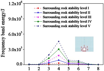
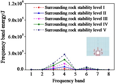
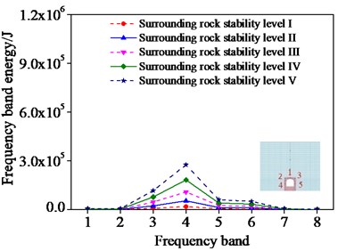
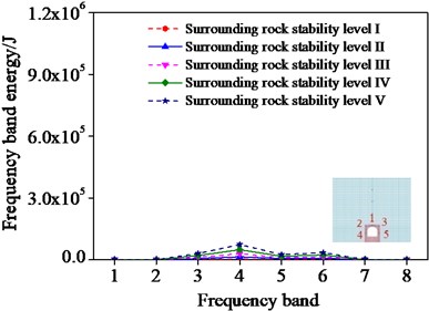
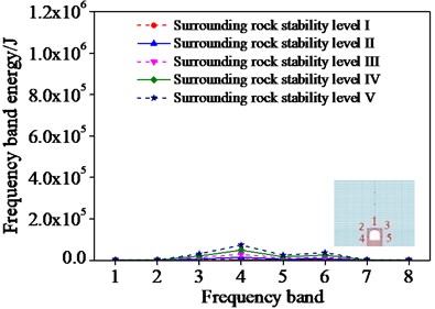
Fig. 8Frequencies band energy of different monitoring points

a) Monitoring point 1

b) Monitoring point 2

c) Monitoring point 3

d) Monitoring point 4

e) Monitoring point 5

In order to analyze the sensitivity of ERVD index to surrounding rock damage, the wavelet-band energy estimation of the surrounding rock with different influencing factors is conducted by setting different monitoring points in different positions of surrounding rocks. A surrounding rock case is selected where five monitoring points are set. And the frequency band energy of the different monitoring points was first computed as shown in Fig. 8.

As shown in Fig. 8, the frequency band energy of different monitoring points increases with the increase of the surrounding rock stability levels. This demonstrates that the frequency band energy increases when the surrounding rock stability decreases. Consequently, the surrounding rock damage degree can be assessed by the change of the frequency band energy.

The frequency band energy of surrounding rock level I is selected as the reference value, and the energy ratio variation deviation of the surrounding rock levels II, III, IV and V can be computed. Twelve surrounding rock cases (Table 5) were selected, besides each surrounding rock sample included five monitoring points. Then, the ERVD of the different monitoring points was computed as shown in Fig. 9.

Fig. 9ERVD of different monitoring points

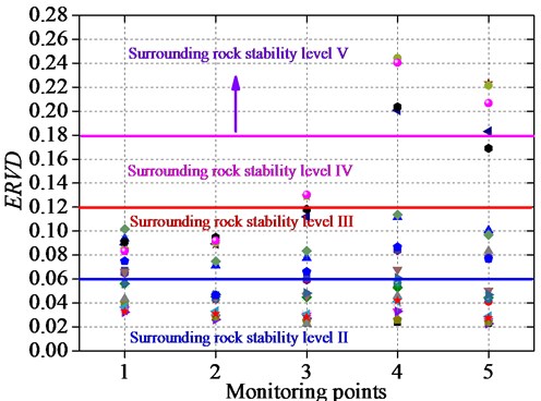
As shown in Fig. 9, the surrounding rock stability levels can be determined by the ERVD index. The ERVD value of the level II ranges from 0 to 0.06; that of the level III ranges from 0.06 to 0.12, and of the level IV ranges from 0.12 to 0.18. The surrounding rock stability level is V when the ERVD is greater than 0.18, which shows that the surrounding rock has a certain failure.

In order to further verify the accuracy of the surrounding rock stability prediction, stress nephograms of the tunnel with different surrounding rock stability levels are given as shown in Fig. 10.

As shown in Fig. 10, it can be found that stress states varied under different surrounding rock stability levels. And the stress of the tunnel surrounding rock with level V is the greatest; it demonstrates that the tunnel surrounding rock with level V is the most unstable. Therefore, the surrounding rock stability prediction can be determined using a stress nephogram by combining with the ERVD index, which can be compared with the results of our proposed prediction model and can confirm the accuracy of the results of our proposed model.

4.3. Surrounding rock stability prediction of tunnel engineering

To assess the surrounding rock stability along the high-speed railway from Jakarta to Bandung in Indonesia, our proposed prediction model which is obtained 30 typical training samples to classify the surrounding rock stability levels was used. And the classified results obtained by our proposed prediction model and finite element method are compared as shown in Table 6.

Fig. 10Stress contour of tunnel with different surrounding rock stability levels

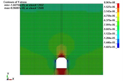
a) Surrounding rock stability level I

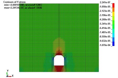
b) Surrounding rock stability level II

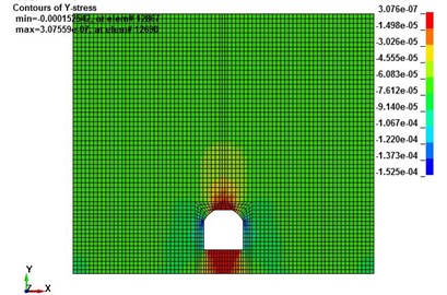
c) Surrounding rock stability level III

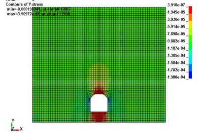
d) Surrounding rock stability level IV

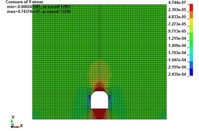
e) Surrounding rock stability level V

As shown in Table 6, our proposed predicted model can be accurately classified in terms of the surrounding rock stability, and is divided into five levels (I, II, III. IV, and V) according to the damage degree, and our proposed prediction model almost achieves the best performance compared to the finite element method. The prediction accuracy is up to 91.67 % which further demonstrates that our proposed prediction model can be used to the surrounding rock stability discrimination for the tunnel engineering hazard safety assessment.

4.4. Surrounding rock stability prediction by laboratory test

To further evaluate the performance of our proposed prediction model based on the KNN algorithm in a surrounding rock stability analysis, a laboratory test which can reproduce the failure process of the tunnel surrounding rock is also conducted to see the prediction performance for different states of the tunnel surrounding rock stability.

Table 6Test samples of surrounding rock stability

No.	RQD	$R_{w}$ (MPa)	$K_{v}$	$K_{f}$	$W$ (L·min^-1)	Finite element result	Our proposed prediction model	Comment
1	0.52	25.0	0.22	0.52	12.0	II	II	Right
2	0.41	25.0	0.22	0.35	12.5	II	II	Right
3	0.28	26.0	0.32	0.30	18.0	III	III	Right
4	0.41	20.0	0.25	0.30	30.0	III	III	Right
5	0.76	132.0	0.78	1.85	3.5	V	V	Right
6	0.20	10.0	0.18	0.19	130.0	IV	IV	Right
7	0.80	100.0	0.58	1.70	8.0	I	III	Fault
8	0.22	13.5	0.10	0.15	135.0	IV	IV	Right
9	0.51	45.0	0.35	0.50	5.0	II	II	Right
10	0.50	40.5	0.38	0.55	10.5	II	II	Right
11	0.24	16.5	0.15	0.15	125.0	V	V	Right
12	0.91	132.0	0.83	0.85	5.5	I	I	Right

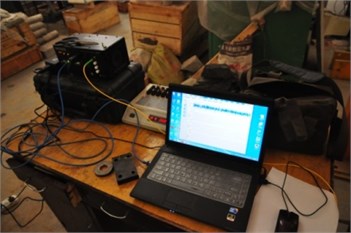
In this experiment, Fiber Bragg Grating (FBG) sensor technology is used to monitor vibration signals during the surrounding rock stability damage. The equipment is Fiber Bragg grating dynamic signal acquisition instrument (SM130), as shown in Fig. 11.

Fig. 11Fiber Bragg grating dynamic signal acquisition instrument

The size of the test model is 1.5 m×1.22 m×0.3 m, and the model is poured in strict accordance with the design ratio. That is, the sand to cement ratio is 5:1. After pouring, standard maintenance is carried out according to the specifications. The simulation of geological structures, such as fault joints, fracture zones and fractures, is a complex problem, and the simulation method is to reduce the modulus and strength of elasticity. In the laboratory test, the stability of tunnel surrounding rock roof is analyzed with the simulation of three stable states of the surrounding rock which is in the stable state, damage state and fail state using three models. And the three stable states refer to surrounding rock stability level I, surrounding rock stability level III and surrounding rock stability level V, respectively. The tunnel surrounding rock models are shown in Fig. 12.

The scaling law between our test model and the real cases follow the Buckingham Pi theorem [25] In our experiment, similar material was developed based on the tunnel material of the high-speed railway from Jakarta to Bandung in Indonesia. The similarity coefficients simulating a tunnel surrounding rock are shown in Table 7.

In the laboratory test, the laboratory test results are compared with our proposed prediction results based on the improved KNN algorithm, and the comparison results are shown in Table 8.

As seen in Table 8, our proposed prediction model based on the improved KNN algorithm achieves the best performance compared to the laboratory test results. The prediction accuracy is up to 100 % that demonstrates that our proposed prediction model can be used for the surrounding rock stability prediction before the tunnel construction.

Fig. 12Tunnel surrounding rock model

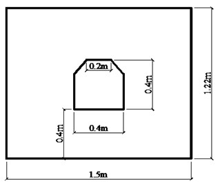
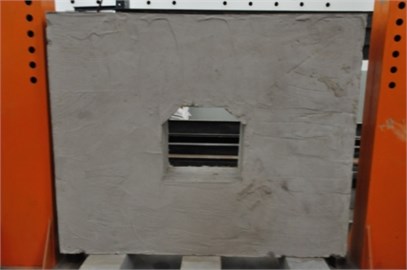
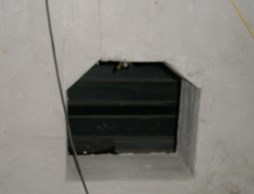
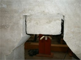
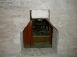
Table 7Similarity coefficients

Physical quantity	Similarity constants
Stress	5
Elasticity modulus	5
Poisson’s ratio	1
Cohesion	1
Unit weight	1
Internal friction angle	1
Displacement	5

Table 8Comparison between laboratory test results and our proposed prediction results

No.	RQD	$R_{w}$ (MPa)	$K_{v}$	$K_{f}$	$W$ (L·min^-1)	Laboratory test result	Our proposed prediction model	Comment
1	0.51	40.2	0.38	0.55	10.5	III	III	Right
2	0.97	180	0.94	0.95	1.3	I	I	Right
3	0.95	160	0.88	0.90	2.5	I	I	Right
4	0.25	15.0	0.20	0.20	125.0	V	V	Right
5	0.13	7.5	0.10	0.10	212.5	V	V	Right
6	0.50	30.0	0.30	0.40	25.0	III	III	Right

5. Conclusions

In our study, a KNN algorithm based on the grouped center vector was proposed, and then a prediction model was established using our improved KNN algorithm, and the prediction model was applied to the surrounding rock stability prediction of a high-speed railway tunnel. Finally, an indoor model experiment was conducted to assess the prediction performance for the surrounding rock stability of the high-speed railway tunnel including stability and instability. Extensive experimental results show that our proposed prediction model achieves much better prediction performance to the surrounding rock stability. The main conclusions are as follows.

1) A prediction model of the surrounding rock stability was proposed based on our improved KNN algorithm, and the experimental results demonstrate that the effectiveness of our proposed prediction model. Our proposed prediction model can be used to assess the damage extent of the tunnel to guide its reinforcement.

2) On the basis of our proposed prediction model, the surrounding rock stability of the tunnels along the high-speed railway is predicted. The surrounding rock stability prediction results between our proposed prediction model and the finite element method match well, and will provide an important contribution to predicting the surrounding rock stability.

3) Laboratory test is conducted for simulating the progressive failure process of the tunnel surrounding rock roof, and the test results show that the prediction accuracy is up to 100 %. This demonstrates that our proposed prediction model can also be used to the surrounding rock stability prediction before the tunnel construction.

References

Deng Shengjun, Lu Xiaomin, Huang Xiaoyang Brief summary of analysis methods for stability of underground surrounding rock masses. Geology and Exploration, Vol. 49, Issue 3, 2013, p. 541-547.

Search CrossRef
Zhang Wenhua Rock prediction recognition of coal mine roadway bolt supporting based on fuzzy mathematical method. Coal Technology, Vol. 32, Issue 6, 2013, p. 74-76.

Search CrossRef
Shao Liangshan, Zhou Yu Prediction on improved GSM-RFC model for cast surrounding rock stability prediction of gateway. Journal of Liaoning Technical University, Vol. 37, Issue 3, 2018, p. 449-455.

Search CrossRef
Wang Yue, Li Longguo, Li Naiwen, Liu Chao Experimental Study on hydraulic characteristics of multi-strand elongated jet impinging into the plunge pool. Yellow River, Vol. 37, Issue 2, 2015, p. 107-110.

Search CrossRef
Wang Jiaxin, Zhou Zonghong, Zhao Ting, et al. Application of Alpha stable distribution probabilistic neural network to prediction of surrounding rock stability assessment. Rock and Soil Mechanics, Vol. 37, Issue 2, 2016, p. 650-657.

Search CrossRef
Qiu Daohong, Li Shucai, Xue Yiguo, et al. Advanced prediction of surrounding rock prediction based on digital drilling technology and QGA-RBF neural network. Rock and Soil Mechanics, Vol. 35, Issue 7, 2014, p. 2013-2018.

Publisher
Yuan Ying, Yu Shaojiang, Wang Chenhui, Zhou Aihong Evaluation model for surrounding rock stability based on support vector machine optimized by grid search method. Geology and Exploration, Vol. 55, Issue 2, 2019, p. 608-612.

Search CrossRef
Li Yidong, Ruan Huaining, Zhu Zhende, et al. Prediction of underground engineering surrounding rock based on improved BP neural network. Yellow River, Vol. 36, Issue 1, 20141, p. 30-133.

Search CrossRef
Li Runqiu, Shi Shilian, Zhu Chuanqu Research on stability prediction of surround rock based on PNN. Mineral Engineering Research, Vol. 28, Issue 3, 2013, p. 30-133.

Search CrossRef
Li Suping, Yao Shuxia Load prediction of HVAC system based on optimization parameter of phase space reconstruction. Refrigeration, Vol. 42, Issue 3, 2013, p. 59-64.

Search CrossRef
Gou Jianping, Qiu Wenmo, Zhang Yi, et al. Locality constrained representation-based K-nearest neighbor prediction. Knowledge-based Systems, Vol. 167, Issue 3, 2019, p. 8-52.

Publisher
Jianping Gou, Hongxing Ma, Weihua Ou, Shaoning Zeng, Yunbo Rao, Hebiao Yang, et al. Generalized mean distance-based k-nearest neighbor classifier. Expert Systems with Applications, Vol. 115, 2019, p. 356-372.

Publisher
Dong Lehong, Geng Guohua, Zhou Mingquan Design of auto text categorization classifier based on Boosting algorithm. Computer Applications, Vol. 27, Issue 2, 2007, p. 384-386.

Search CrossRef
Jianping Gou, Wenmo Qiu, Zhang Yi, et al. Local mean representation-based K-nearest neighbor classifier. ACM Transactions on Intelligent Systems and Technology, Vol. 10, Issue 3, 2019, p. 29.

Search CrossRef
Dudani S. A. Distance-weighted k-nearest-neighbor rule. IEEE Transactions on Systems, Man, and Cybernetics, Vol. SMC-6, Issue 4, 1976, p. 325-327.

Publisher
Jianping Gou, Lan Du, Yuhong Zhang, et al. New distance-weighted k-nearest neighbor classifier. Journal of Information and Computing Science, Vol. 9, Issue 6, 2012, p. 1429-1436.

Search CrossRef
Junfei Zheng Improvement on feature selection and prediction algorithm for text prediction. Xidian University, Xi An, 2012.

Search CrossRef
Liu Shuchang Zhang Zhonglin Multi-stage prediction KNN algorithm based on center vector. Computer Engineering and Science, Vol. 39, Issue 9, 2017, p. 1758-1764.

Search CrossRef
Wang Jun Yao Study of Application of Text Prediction Techniques on Weibo. Guangxi University Nanning, 2015.

Search CrossRef
Bao Xuechao Research on Chinese Automatic Text Categorization Based on Support Vector Machine. Shanghai Jiao Tong University, Shang Hai, 2005.

Search CrossRef
Li Xianbin Prediction of stability of surrounding rock based on PCA-logistic model Yellow River, Vol. 37, Issue 2, 2015, p. 106-114.

Search CrossRef
China Electricity Council. GB 50287-2006 Code for Hydropower Engineering Geological Investigation. China Planning Press, Beijing, 2006.

Search CrossRef
Zhang Wei, Li Xibing, Gong Fengqiang Stability prediction model of minelane surrounding rock based on distance discriminant analysis method. Journal of Central South University of Technology, Vol. 15, Issue 1, 2008, p. 117-120.

Publisher
Seo J. H., Yong H. L., Kim Y. H. Feature selection for very short-term heavy rainfall prediction using evolutionary computation. Advances in Meteorology, Vol. 2014, 2014, p. 203545.

Publisher
Louis B. Pi theorem of dimensional analysis. Archive for Rational Mechanics and Analysis, Vol. 1, Issue 1, 1957, p. 35-45.

Publisher

Cited by

Predicting structure performance of urban critical infrastructure: an augmented attention-based LSTM model

(2024)

Application of CPT test in the evaluation of the test effect of lime soil compacting pile

Wenqiang Li

(2023)

Q-method optimization of tunnel surrounding rock classification by fuzzy reasoning model and support vector machine

(2022)

Multi-class object detection in tunnels from 3D point clouds: An auto-optimized lazy learning approach

Kunyu Wang | Zhaoxiang Zhang | Xianguo Wu | Limao Zhang

(2022)

2022 8th International Conference on Hydraulic and Civil Engineering: Deep Space Intelligent Development and Utilization Forum (ICHCE)

Penggang Zhu

(2022)

Study on control measures of the influence of shallow buried tunnel excavation on the subgrade settlement of high speed railway in operation

Qiyu Song

(2021)

About this article

Received

20 April 2020

Accepted

15 August 2020

Published

15 November 2020

SUBJECTS

Seismic engineering and applications

DOI

https://doi.org/10.21595/jve.2020.21427

Keywords

tunnel

surrounding rock stability

K-nearest neighbor algorithm

grouped center vector

prediction model

Acknowledgements

This work is financially supported by the National Natural Science Foundation of China (Grant No. 51708516), as per the Young Elite Scientists Sponsorship Program by CAST (2018QNRC001), Project from China Coal Industry Group Co., Ltd (2019-2-ZD004) and (2019-2-ZD003) and Beijing Municipal Natural Science Foundation (8174078).

This is an open access article distributed under the Creative Commons Attribution License, which permits unrestricted use, distribution, and reproduction in any medium, provided the original work is properly cited.

Previous article in issue Previous Next article in issue Next

Research article

2023 08 03

Determining tunnel stability across fault zones under seismic loading based on load/unload response ratio theory

Qiang Hui, Feng Gao, Xukai Tan, Dongmei You

Research article

2023 06 26

Prevention of Large Deformation of Soft Surrounding Rock in Tunnel Construction

Xiaoqing Suo, Feng Gao, Bo Hu, Xuefu Zhang, Rui Qu

Research article

2023 06 26

Longitudinal deformation of Shield tunnel based on construction monitoring data

Wenkang Yao

Research article

2023 04 09

Dynamic damage and response characteristics of the tunnel by FEM modeling and field trials

Xianjun Zheng, Tingyao Wu, Chao Wu, Xiaoqin Wang

S. Huang, Q. Qi, J. Liu, and W. Liu, “Tunnel surrounding rock stability prediction using improved KNN algorithm,” Journal of Vibroengineering, Vol. 22, No. 7, pp. 1674–1691, Nov. 2020, https://doi.org/10.21595/jve.2020.21427

Copy Extrica

Copied to clipboard!

TY  - JOUR
DO  - 10.21595/jve.2020.21427
UR  - https://doi.org/10.21595/jve.2020.21427
TI  - Tunnel surrounding rock stability prediction using improved KNN algorithm
T2  - Journal of Vibroengineering
AU  - Qi, Qingjie
AU  - Huang, Shuai
AU  - Liu, Jianzhong
AU  - Liu, Wengang
PY  - 2020
DA  - 2020/11/15
PB  - JVE International Ltd.
SP  - 1674-1691
IS  - 7
VL  - 22
SN  - 1392-8716
SN  - 2538-8460
ER  - 

Copy Ris

Copied to clipboard!

@article{Qi_2020,
	doi = {10.21595/jve.2020.21427},
	url = {https://doi.org/10.21595/jve.2020.21427},
	year = 2020,
	month = {nov},
	publisher = {{JVE} International Ltd.},
	volume = {22},
	number = {7},
	pages = {1674--1691},
	author = {Qingjie Qi and Shuai Huang and Jianzhong Liu and Wengang Liu},
	title = {Tunnel surrounding rock stability prediction using improved {KNN} algorithm},
	journal = {Journal of Vibroengineering}
}

Copy Bibtex

Copied to clipboard!

[1]Q. Qi, S. Huang, J. Liu, and W. Liu, “Tunnel surrounding rock stability prediction using improved KNN algorithm,” Journal of Vibroengineering, vol. 22, no. 7, pp. 1674–1691, Nov. 2020, doi: 10.21595/jve.2020.21427.

Copy IEEE

Copied to clipboard!

Qi, Qingjie, Shuai Huang, Jianzhong Liu, and Wengang Liu. “Tunnel Surrounding Rock Stability Prediction Using Improved KNN Algorithm.” Journal of Vibroengineering 22, no. 7 (November 15, 2020): 1674–91. https://doi.org/10.21595/jve.2020.21427.

Copy Chicago

Copied to clipboard!

Tunnel surrounding rock stability prediction using improved KNN algorithm

Abstract

Highlights

1. Introduction

2. Our improved KNN algorithm

2.1. KNN, WKNN and DWKNN

2.2. Support vector machine (SVM) [20]

2.3. Our improved KNN algorithm

3. Surrounding rock stability prediction based on our improved KNN algorithm

3.1. Influencing factors and surrounding rock stability prediction

3.2. Normalization

3.3. Criteria for our prediction approach performance

3.4. Prediction of surrounding rock stability

4. Engineering application of our proposed prediction model

4.1. Finite element model of tunnel surrounding rock

4.2. Evaluation index of surrounding rock stability

4.3. Surrounding rock stability prediction of tunnel engineering

4.4. Surrounding rock stability prediction by laboratory test

5. Conclusions

References

Cited by

About this article

Related Articles