Mathematical simulation of adaptive vector finite element method for the analysis of electromagnetic vibration spectrum field response

Cheng, Yiyuan; Su, Mingyang; Hui, Ming; Liu, Wei; Zheng, Yangbing

doi:10.21595/jve.2021.22031

Journal of Vibroengineering

Browse Journal

Submit article

Published: 30 September 2021

Check for updates

Mathematical simulation of adaptive vector finite element method for the analysis of electromagnetic vibration spectrum field response

Yiyuan Cheng¹

Mingyang Su²

Ming Hui³

Wei Liu⁴

Yangbing Zheng⁵

^{1, 4, 5}Department of Mechanical and Electrical Engineering, Nanyang Normal University, Nanyang, Henan, 473061, China

²Department of Environmental Engineering, Henan Polytechnic Institute, Nanyang, Henan, 473000, China

³Department of physics and Electronic Engineering, Nanyang Normal University, Nanyang, Henan, 473061, China

Corresponding Author:

Yiyuan Cheng

Cite the article Download PDF

Downloads 615

Abstract

Mathematical simulation plays a vital role in the analysis of electromagnetic vibration spectrum field response. This article realizes a three-dimensional adaptive vector finite meta-acting algorithm of controlled source electromagnetic vibration spectrum (CSEM) field to address 3D meshing for the simulation of terrain fluctuations and complex electrical anomalies. The adaptive methods utilized in this article is employed for one-time field and secondary field separation in order to calculate electromagnetic vibration spectrum field response. This response can effectively solve the source singularity in finite meta-simulation and improves the numerical accuracy of electromagnetic vibration spectrum field near the field source. The two approaches analysed in this article are CSEM one-dimensional positive algorithm and finite meta-method. The adaptive mesh refinement algorithm based on post-test error estimation is used in this paper to guide the mesh refinement to reduce man-made errors caused by designing a grid. The validity of the proposed algorithm is verified through numerical simulation of one-dimensional and three-dimensional models. The outcomes obtained reveals that the finite solution of one-dimensional model coincides well with the analytical solution. The relative error of electromagnetic vibration spectrum field amplitude is about 1 %, and the overall phase difference of less than 1 degree is observed. It is analysed that the three-dimensional model finite solution also fits well with the finite volume solution and the controlled source electromagnetic vibration spectrum response with three-dimensional tilt plate abnormality is simulated. This experimental analysis shows the ability and effectiveness of the algorithm to simulate the electromagnetic vibration spectrum field of complex geoelectrical structure.

Mathematical simulation of adaptive vector finite element method for the analysis of electromagnetic vibration spectrum field response

Highlights

The three-dimensional positive calculation of controlled source electromagnetic vibration spectrum field is realised based on the finite meta-method utilizing the non-structural mesh vector and adaptive mesh refinement technology.
The 3D meshing for the simulation of terrain fluctuations and complex electrical anomalies is addressed in this article by proposing a three-dimensional adaptive vector finite meta-acting algorithm of controlled source electromagnetism (CSEM).
An adaptive vector finite element algorithm is used to realize the CSEM3D forward simulation and the primary/secondary field separation algorithms are utilized for the calculation of the electromagnetic vibration spectrum field response.
The controlled source electromagnetic response with three-dimensional tilt plate abnormality is simulated by using this algorithm.

1. Introduction

In the exploration of ground electromagnetic vibration spectrum method, controllable source audio geomagneance method (CSAMT) plays an important role in the survey and exploration of petroleum, geothermal, metal mineral, hydration, environment and so on. Ocean controlled source electromagnetic vibration spectrum method (CSEM) is a new method of marine geophysical exploration, which can help seismic methods to identify effective reservoirs and improve drilling success rate. Marine CSEM technology has been widely used in the exploration of marine oil and gas resources, and has achieved remarkable results. In controllable source electromagnetic vibration spectrum method, the source, field and observation system are all three-dimensional in essence, and solving the three-dimensional problem is the most important way to improve the reliability and resolution of data [1-3].

In recent years, great progress has been made in the study of the three-dimensional forwarding method of controllable source electromagnetic vibration spectrum field, and many equations based on integral equations have been proposed. Most of these algorithms are implemented on the structural grid, but the structural grid cannot accurately simulate complex geological structures such as terrain fluctuations and tilt interfaces, and the non-structural mesh finite meta-method is more suitable for simulating these complex geo-electronic models, and the completely non-structural mesh can realistically simulate complex geological structures such as terrain ups and downs and tilt interfaces, especially non-structural [4, 5]. Lipinski P. et al. developed a simplified linear model of WiFi electromagnetic vibration spectrum field modeling and compared it with the most commonly used, more complex models and the measurements performed in the lab. As demonstrated by measurements made using various hardware, the accuracy of this simplified model introduced is similar to that of common models, but the number of parameters is small. As a result, our model is easier to implement in real life. When the exact value of propagation parameters and transmitter characteristics is unknown, the model presented in this paper can be used to model WiFi electromagnetic vibration spectrum fields. This is often the case in the early stages of structural network design, and the exact parameters of building materials are not yet known. Because the model is so simple, it does not require much deployment work and is accurate enough to meet the initial positioning requirements of WiFi transmitters. A simplified model of WiFi electromagnetic vibration spectrum field propagation is known, but there has been no comparative study of combining measurement with measurement in this field. This paper provides a comparison of different electromagnetic vibration spectrum field models that can be applied to WiFi electromagnetic vibration spectrum field propagation together with the measurement results [6]. Kumar P. et al. are very useful in studying electromagnetic vibration spectrum fields and non-ionization effects on the human body. When an electric field or magnetic field penetrates the body, it is weakened and a portion of it is absorbed into the body’s tissues. The effect of EM on the human body depends on the strength of the electromagnetic vibration spectrum field and the distance from the EM source to the human body. The ratio absorption rate (SAR) is a parameter used to estimate the amount of energy absorbed by the body. THE SAR depends on frequency and strength, electromagnetic vibration spectrum wave. Extensive research has been done to reduce SAR use in mobile phones, but minimizing SAR in medical applications such as MRI has always been a challenge for researchers. The advantages of magnetic resonance imaging (MRI) make it a radiological option for a large number of analytical procedures, but the disadvantage is that for patients with implantable devices, the choice is limited and the SAR value increases due to higher temperatures for implantable devices. Magnetic field leaks from diagnostic instruments can pose a risk to medical personnel. This paper is based on the preliminary work of SAR research on the basis of considering electromagnetic vibration spectrum wave intensity and evaluating SAR in the case of magnetic field leakage [7]. Hasan S. et al. have proposed a control strategy that uses the reactive power support based on voltage feedback from existing Distributed Generators (DGs) to minimize the impact of induction motor start-up on network voltage. Simulation research is proposed to validate the theoretical framework. The results show that DG can quickly restore the motor's start-up transient voltage drop due to the rapid response of the voltage controller designed for DG [8]. The impact of motor starting is analysed by Afrin, et al. [9] on the micro grid in order to assess the network distribution of instantaneous heavy load. Medina, et al. [10] and Nujaimi, et al. [11] proposed an evaluation technique in order to assess the network distribution reliability in the conditions of cold load. The induction motor impact over the network was minimised by Kumar, et al. [12] and Widiputra and Jung [13] using the voltage feedback control strategy. Li, et al. [14] evaluated the impact of heavy load on the distributor networks using energy storage and photovoltaic capacitor method in order to verify the analysis. Various researchers have made an attempt in order to achieve the load recovery for the distribution network while imposing the instantaneous heavy load conditions [15-17]. But a reliable and efficient solution is not achieved using the current state of the art methods.

This paper realizes the three-dimensional positive calculation of controlled source electromagnetic vibration spectrum field based on the finite meta-method utilizing the non-structural mesh vector and adaptive mesh refinement technology [18-20]. The 3D meshing for the simulation of terrain fluctuations and complex electrical anomalies is addressed in this article by proposing a three-dimensional adaptive vector finite meta-acting algorithm of controlled source electromagnetic vibration spectrum (CSEM) field. An adaptive vector finite element algorithm is used to realize the CSEM3D forward simulation and the primary/secondary field separation algorithms are utilized for the calculation of the electromagnetic vibration spectrum field response. The controlled source electromagnetic response with three-dimensional tilt plate abnormality is simulated by using this algorithm and the numerical solutions of analytical solution and three-dimensional finite volume method are compared and analysed. The outcomes obtained reveals the ability and effectiveness of the algorithm to simulate electromagnetic vibration spectrum field of complex geoelectrical structure [21-23]. The algorithms utilized in this article can calculate the electromagnetic field of a galvanic source with a finite length in any posture, and the source and receiving points can be placed in any position, providing good versatility.

The rest of this article is organised as: The description of unstructured grid vector finite element method is given in Section 2 followed by the explanation of adaptive mesh refinement algorithm based on posterior error estimation in Section 3. Results and analysis of the numerical simulation are presented in Section 4 which is trailed by the concluding remarks in Section 5.

2. Unstructured grid vector finite element method

2.1. Governing equation

Assuming the time factor is $e^{- i ω t}$ , in the quasi-steady state, the governing equations satisfied by the electric field ( $E$ ) and the magnetic field ( $H$ ) are:

1

\begin{array}{l} \nabla \times E - i ω μ_{0} H = 0, \\ \nabla \times H - σ E = J, \end{array}

where $μ_{0}$ is the magnetic permeability in vacuum, $ω$ is the angular frequency, $J$ is a current source, $σ$ is the conductivity. In order to eliminate the singularity of the electromagnetic vibration spectrum field near the source point, the electromagnetic vibration spectrum field is decomposed into $σ^{p}$ the primary field ( $E^{p}$ with $H^{p}$ ) and conductivity $σ^{s} = σ - σ^{p}$ the secondary field produced by the anomalous body ( $E^{s}$ with $H^{s}$ ). The primary field can be obtained by the pseudo-analytical method [24-26].

The secondary electromagnetic vibration spectrum field satisfies the following equation:

2

\begin{array}{l} \nabla \times E^{s} - i ω μ_{0} H^{s} = 0, \\ \nabla \times H^{s} - σ E^{s} = σ^{s} E^{p} . \end{array}

From Eq. (2), it can be deduced that the secondary electric field $E^{s}$ partial differential equation:

3

\nabla \times \nabla \times E^{s} - i ω μ_{0} E^{s} = i ω μ_{0} σ^{s} E^{p} .

We use the finite element method to solve Eq. (3). When the secondary electric field is obtained $E^{s}$ after that, the secondary magnetic field can be calculated using Eq. (4):

4

H^{s} = \frac{\nabla \times E^{s}}{i ω μ_{0}} .

2.2. Finite element analysis

Using the weighted residual method, the integral equation corresponding to the partial differential Eq. (3) can be derived. Multiply the left and right sides of Eq. (3) by any variation of the electric field $δ E^{s}$ , and integrate the simulation area $Ω$ , combined with the divergence formula and green's theorem, we can get:

5

\begin{matrix} \int_{Ω} [(\nabla \times δ E^{s}) \cdot (\nabla \times E^{s}) - δ E^{s} \cdot i ω μ_{0} σ E^{s}] d Ω = \int_{Ω} i ω μ_{0} σ E^{s} σ^{s} E^{p} d Ω . \end{matrix}

Assume that the secondary electric field satisfies the homogeneous boundary condition on the outer boundary of the simulation area:

6

n \times E^{s} = 0 .

The finite element Eq. (5) can be solved by the conventional nodal finite element method and the vector finite element method, but when the nodal finite element method is used, the continuous boundary condition of the normal component of the electric field and the condition that the electromagnetic vibration spectrum field divergence is zero cannot be guaranteed. As a result, false solutions may appear, and the processing of curl operators and the application of boundary conditions are more troublesome. Eq. (5) can be obtained through a certain transformation to obtain the electromagnetic vibration spectrum potential equation under the coulomb gauge or the Lorentz gauge. Solving the electromagnetic vibration spectrum potential avoids the normal discontinuity of the electric field in the earth's medium. It can be solved directly by the nodal finite element method. However, because the interpolation function of the nodal finite element does not satisfy the condition of zero divergence, a false solution will be generated, and the accuracy of the numerical simulation will obviously be reduced when the electromagnetic vibration spectrum potential is solved first and then the electromagnetic vibration spectrum field is solved by the difference scheme. The vector finite element method can overcome the above problems [27, 28].

Fig. 1Schematic diagram of tetrahedral element nodes and vector edges

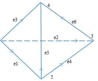
We use unstructured tetrahedral elements to discretize the simulation area. Fig. 1 shows a tetrahedral element with 4 nodes and 6 edges. Assume that the tangential component of the electric field on the edge is $E_{i} (i = 1, . . ., 6)$ , and the direction of the tangential component of the electric field at the midpoint of the edge is consistent with the direction of the edge. The electric field at any point in the unit can be obtained by linear interpolation of the electric field on the 6 edges in the unit:

7

E = \sum_{i = 1}^{6} N_{i} E_{i},

where $N_{i}$ it is a linear interpolation basis function. We use nédélec type vector basis functions:

8

N_{i} = l_{i} (L_{i 1} \nabla L_{i 2} - L_{i 2} \nabla L_{i 1}),

where $l_{i}$ is the length of the $i$ th side, $L_{i 1}$ , $L_{i 2}$ are the starting points of the $i$ th edge $i_{1}$ and the end $i_{2}$ the node basis function. Correct $N_{i}$ take the divergence, get $\nabla \cdot N_{i} = 0$ , that is, the nédélec-type vector basis function satisfies the condition of zero divergence [29].

Substituting Eq. (7) into integral Eq. (5), and calculating the unit integral, we can get:

9

δ E^{s} (\sum_{1}^{n e} K_{1}^{e} + K_{2}^{e}) E^{s} = δ E^{s} \sum_{1}^{n e} p^{e},

among them, $n e$ is the number of tetrahedral units:

10

K_{1}^{e} = \int_{Ω_{e}} [{(\nabla \times N)}^{T} \cdot (\nabla \times N)] d Ω,

11

K_{2}^{e} = - i ω μ σ \int_{Ω_{e}} [N^{T} \cdot N] d Ω,

12

P_{}^{e} = - i ω μ_{0} σ^{s} \int_{Ω_{e}} [N^{T} \cdot E^{p}] d Ω .

Consider the variation $δ E^{s}$ the arbitrariness of, the finite element linear equations can be obtained from Eq. (9), and the linear equations can be solved by the direct method to obtain the quadratic field, and then add to the primary field vector to obtain the total electromagnetic vibration spectrum field.

3. Adaptive mesh refinement algorithm based on posterior error estimation

Eq. (5) can be expressed as:

13

B (u, v) = F (v),

among them:

14

B (u, v) = \int_{Ω} [(\nabla \times u) \cdot (\nabla \times v) - k^{2} u v] d Ω,

F (v) = \int_{Ω} i ω μ σ^{s} E^{p} v d Ω,

where $k^{2} = i ω μ σ$ .

Assume that the function $G$ is the exact solution u of the electromagnetic vibration spectrum field and the finite element numerical solution $u_{h}$ error of $u - u_{h}$ the functional of Eq. (13) is:

15

B^{*} (w, v) = G (v),

among them, $B^{*}$ it is a dual or adjoint operator. Assume $B^{*} (w, v) = B (v, w)$ , then there are:

16

G (u - u_{h}) = B^{*} (w, u - u_{h}) = B (u - u_{h}, w) = B (u - u_{h}, w - w_{h}),

where $w$ and $w_{h}$ they are the exact solution of the dual problem and the finite element numerical solution.

According to Eq. (14), the right term of dual Eq. (15) is:

17

G (v) = \frac{1}{{‖\nabla \times u‖}_{L^{2} (Ω)}^{2}} (\int_{Ω} (f + k^{2} u) \cdot v - (\nabla \times u) \times (\nabla \times v) d Ω

- \int_{\partial Ω} ((\nabla \times u) \times n) \cdot v d S .

Among them, $Ω$ is the continuous area containing the receiving point, $\partial Ω$ is the boundary of the continuous region, and $v$ is an arbitrary vector. Solving Eq. (15) can obtain the finite element solution of the dual problem $ω_{h}$ .

Define a posterior error estimate based on residuals and dual weighting:

18

η = η_{τ} (u) η_{τ} (w),

among them:

19

η_{τ}^{2} (u) = h^{2} ({‖R_{1} (u)‖}^{2} + {‖R_{2} (u)‖}^{2}) + h \sum_{f \in Ω} ({‖J_{1} (u)‖}^{2} + {‖J_{2} (u)‖}^{2}),

20

\begin{array}{l} R_{1} (u) = (f + k^{2} u - (\nabla \times \nabla \times u)), \\ R_{2} (u) = \nabla \cdot (f + k^{2} u), \\ J_{1} (u) = (\nabla \times u) \times n, \\ J_{2} (u) = (f + k^{2} u) \cdot n . \end{array}

In the formula, $h$ is the diameter of the circumcircle of the tetrahedron. $η_{τ} (w)$ calculation formula and $η_{τ} (u)$ similar.

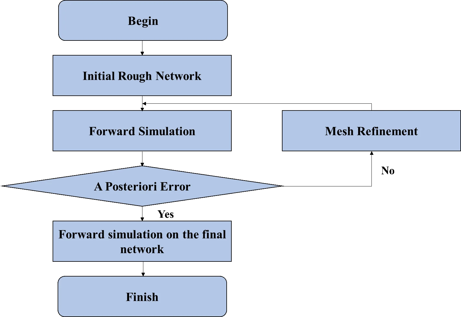
Fig. 2The calculation process of the adaptive finite element algorithm

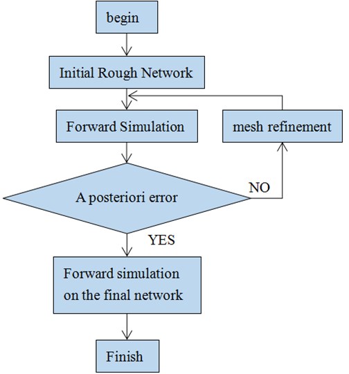
The steps of the adaptive finite element algorithm are as follows:

1. Given an initial coarse mesh, use the finite element method to solve Eq. (13) to obtain its finite element solution.

2. Solve the dual problem finite element Eq. (15), obtain the finite element solution to the dual problem.

3. Calculate the posterior error of each element according to Eq. (18), and refine the elements with a large error in a certain proportion (the calculation examples in this paper are set to 5 % of the total number of elements). Get a new mesh.

4. Repeat steps (1)-(3) until the root mean square error of the finite element solution before and after mesh refinement meets the accuracy requirements or reaches the set maximum mesh refinement times. The specific process is shown in Fig. 2 [16].

4. Results and analysis of the numerical calculation

4.1. One-dimensional oil and gas model

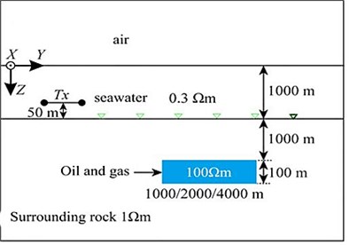
In order to verify the correctness of the algorithm and program, the 1D model shown in Fig. 3 is designed. Assume that the seawater resistivity is 0.3 Ωm and the seawater depth is 1000 m; the bottom of the seabed is a 1000 m thick overburden with a resistivity of 1 Ωm; the bottom of the overburden is A 500 m thick high-resistance oil and gas layer with a resistivity of 100 Ωm; below the oil and gas layer is a formation with a resistivity of 1 Ωm; the galvanic source is arranged 50 m above the seabed, and its center point is (0 m, 0 m, 950 m), and the length it is 1m, the emission current is 1 A, and the emission frequency is 0.25 Hz. Assume that a total of 20 receiving points are along the survey line direction ( $X =$ 0), and are evenly arranged on the seabed at equal intervals within the range of $Y =$ 500-10000 m [30].

Fig. 31D oil and gas model

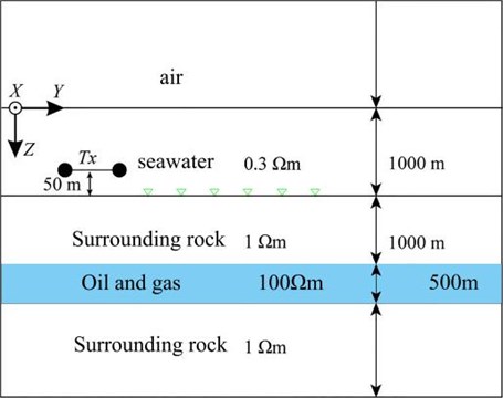
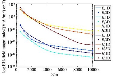
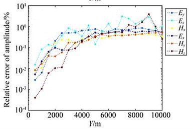
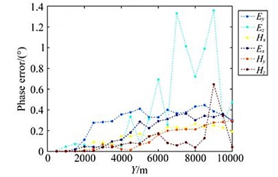
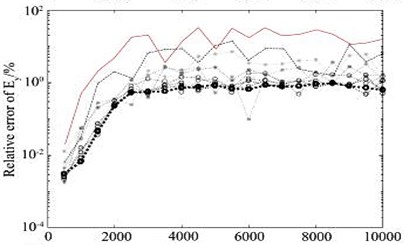
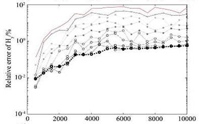
Fig. 4 shows the comparison between the adaptive finite element solution and the 1D analytical solution.

The corresponding curve in the figure is the result of the source being arranged in the $X$ direction, and the corresponding curve is the result of the source being arranged in the $Y$ direction. It can be seen that the relative amplitude error of the horizontal electromagnetic vibration spectrum field component is less than 1 %, and the phase difference is within 1°. For the vertical electromagnetic vibration spectrum field component, when the transmission distance is small (less than 5 km), the relative amplitude error is less than 1 %, and the phase difference is 1° when the transmission distance is greater than 5 km, the relative error of the amplitude is relatively large, and the maximum phase difference of the components is 1.4°.

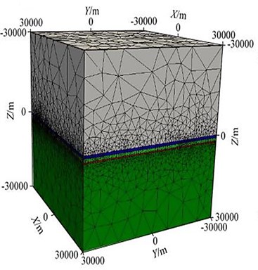
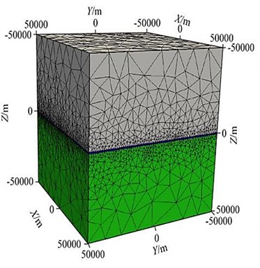
The finite element simulation area is 60 km×60 km×60 km, the initial grid is shown in Fig. 5(a), and the grid of the part of interest in the grid is extracted (Fig. 5(b)) (0 km $< X <$ 1 km, –0.5 km $< Y <$ 10.5 km, –0.5 km $< Z <$ 3 km), it can be seen that the initial grid is very rough, and the grids of the transmitting source and receiving points are not refined.

Fig. 4Comparison of adaptive finite element solution and analytical solution (1D Oil and Gas Model)

(a)

(b)

(c)

(d)

Fig. 5Grid schematic (1D oil and gas model)

a)

b)

c)

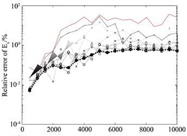
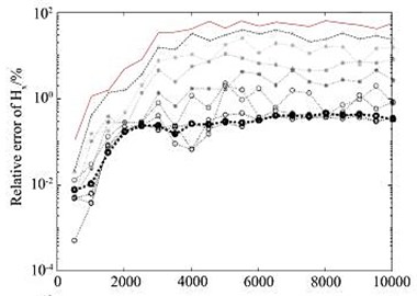
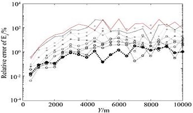
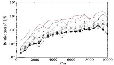
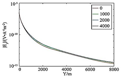
After 10 times of mesh refinement, the final mesh obtained is shown in Fig. 5(c). It can be seen from the figure that in the area near the receiving point, the grid is well encrypted, and the grid below the receiving point is also refined to a certain extent, thus ensuring the accuracy of the numerical solution. In the finite element numerical simulation, if you want to obtain a high-precision numerical solution, the finite element mesh needs to be discretized sufficiently fine. The adaptive mesh refinement algorithm uses the posterior error estimation method to estimate the accuracy of the finite element numerical solution, and gradually refines the mesh with larger errors, thereby ensuring the rationality of the mesh refinement. Each time the number of meshes involved in the refinement cannot be too small, too small will require more refinement times; but not too much, too much will also refine the meshes with small errors, thereby increasing calculation amount. After many simulation tests, some units with larger errors (5 % of the total number of units) are refined, and the effect is the best. Fig. 6 shows the change of the relative error of the electromagnetic vibration spectrum field amplitude during the adaptive mesh refinement process.

Fig. 6Changes of relative error of electromagnetic vibration spectrum field amplitude during adaptive mesh refinement

a)

b)

c)

d)

e)

f)

It can be seen from the figure that the relative error of the numerical solution amplitude obtained on the initial grid (part of the area shown in Fig. 5(b)) is basically more than 10 %, but as the number of refinements increases, the relative error of the electromagnetic vibration spectrum field amplitude gradually decreases, after 10 times after the mesh is refined (part of the area is shown in Fig. 5(c)), the relative error of the amplitude basically converges to about 1 %.

In the mesh refinement process of the above calculation example, it is theoretically required to refine only 5 % of the total number of cells each time. However, because the meshing software is based on the delaunay meshing algorithm, it may be refined each time the number of grid cells is greater than 5 %. Table 1 details the number of grid cells, the number of edges, CPU time, solver time, memory consumption, primary field time and RmS during the mesh refinement process. Among them, RmS is the root mean square error between the calculation result of each iteration and the calculation result of the previous iteration. It can be seen from the table that when the number of grids is small, the calculation time of one field accounts for the main part, but when the number of grids becomes more and more when it is large, the calculation time required to solve the linear equations becomes longer and longer. After 10 iterations, RmS converges to 1.0 [31].

4.2. Three-dimensional oil and gas model

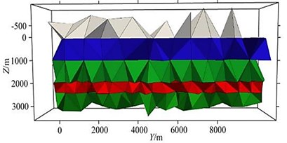
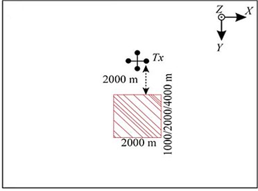
Establish a three-dimensional ocean oil and gas reservoir model as shown in Fig. 7.

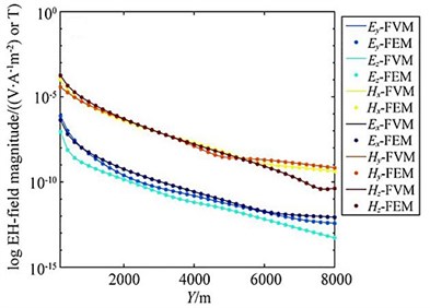
Assume that the seawater resistivity is 0.3 Ωm and the seawater depth is 1000 m; there is a 100 m thick high-resistance oil and gas layer at a depth of 1000 m under the seafloor, and its resistivity is 100 Ωm. The direction length is 2000 m, and the distribution range is [–1000, 1000] m; three different lengths are designed in the $Y$ direction, and the distribution ranges are [2000, 3000] m, [2000, 4000] m and [2000, 6000] m. Surrounding the thin oil and gas layer is the surrounding rock with a resistivity of 1 Ωm; the galvanic source is arranged 50 m above the seabed, and its center point is (0 m, 0 m, 950 m), the length is 100 m, the emission current is 1 A, and the frequency is 0.25 Hz; A total of 41 receiving points along the survey line direction ( $X =$ 0) are evenly arranged on the seabed at equal intervals within the range of 0 m and 8 km. In order to further verify the correctness of the algorithm, the adaptive vector finite element algorithm in this paper and the marine controllable source electromagnetic vibration spectrum three-dimensional forward algorithm based on the staggered grid finite volume (FVM) method are used to simulate the electromagnetic vibration spectrum field response of the three-dimensional model shown in Fig. 7. Fig. 8 shows the simulation results of the two algorithms.

Fig. 7Three-dimensional offshore reservoir model

a)

b)

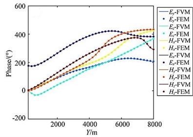
In the figure, the $E_{x}$ , $H_{y}$ , and $H_{z}$ curves are the results of the source arranged in the $X$ direction, and the $E_{Y}$ , $E_{Z}$ , $H_{X}$ curves are the source arranged in the $Y$ direction. Result. It can be seen from the figure that the amplitude curve and phase curve overlap very well. The entire simulation area is 100 km×100 km×100 km (taking a example of a 2 km×2 km oil and gas reservoir model.

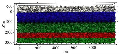
The initial grid is shown in Fig. 9(a). Although the grid area is very large, the cells near the outer boundary are very large; the area of interest in the extracted grid is displayed separately as shown in Fig. 9(b) (0 km $< X <$ 1 km, -0.5 km $< Y <$ 8.5 km, -0.5 km $< Z <$ 2.5 km).

Fig. 8Comparison of adaptive finite element solution with finite volume method (3D oil & gas model)

a)

b)

Fig. 9Grid schematic (3D oil and gas model)

a)

b)

c)

It can be seen that the initial grid is very rough, and there is no refinement of the grid of the emission source, the receiving point and the oil and gas reservoir area; after 15 grid refinements, it converges, and the grids in some areas the refinement is shown in Fig. 9(c), and there is good encryption near the receiving point and the oil and gas reservoir area, which ensures the accuracy of the numerical solution.

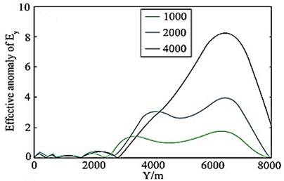
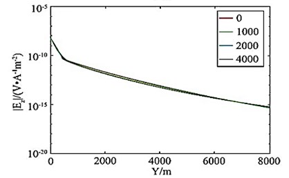
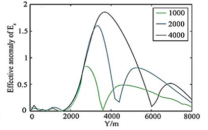
Analysis of the electric field curve of the horizontal thin plate-shaped high-resistance oil and gas reservoir model found that only when its horizontal size is at least 2 times the buried depth, can it be distinguished by CSEM. At present, the commonly used qualitative interpretation method of marine CSEM data it is to calculate the ratio of the electromagnetic vibration spectrum field amplitude of the reservoir containing oil and gas; to the electromagnetic vibration spectrum field amplitude of the background model using the reservoir without oil and gas, called the normalized field. Taking the interference factors such as observation error and noise into account, calculate the electromagnetic vibration spectrum field amplitude of the target model and the background model the ratio of the difference to the background noise is used to measure the size of the anomaly, which is called the effective anomaly. The calculation formula is:

21

Δ = \frac{||E_{M}| - |E_{O}||}{E_{n o i s e}},

22

E_{n o i s e} = \sqrt{E_{r e l}^{2} + E_{r o t}^{2} + E_{a b s}^{2}},

among them, $|E_{M}|$ is the electric field amplitude of the reservoir model containing oil and gas; $|E_{o}^{}|$ is the electric field amplitude of the background model without oil and gas reservoirs; $|E_{n o i s e}|$ is electric field noise; $E_{r e l}$ is the relative error of the amplitude, including the error generated by the instrument system and the observation error; $E_{a b s}$ is the absolute error, is the noise floor of the transmitting-receiving system, usually taken $E_{a b s} = 1 0^{- 16} V \cdot A^{- 1} m^{- 2}$ ; $E_{r o t}$ it is the error caused by the rotation angle of the receiving station, and the rotation angle error is taken here as 5°. Figs. 10(a) and 10(b) are the different lengths in the marine oil and gas reservoir model (Fig. 7) (the length in the $Y$ direction is 0 m respectively (that is, the oil and gas reservoirs are not included). (1 km, 2 km, 4 km) of the horizontal electric field EY amplitude curve and effective abnormal curve, Fig. 10(c) and 10(d) correspond to the amplitude curve and effective abnormal curve of the vertical electric field EZ respectively. It can be seen that if you only look at the amplitude curve, it is difficult to distinguish the anomaly of the horizontal electric field with a length of 1 km and 2 km in the oil and gas reservoir, but the anomaly in the effective anomaly curve (Fig. 10(b), 10(d)) is more obvious, especially the effective anomaly calculated by the vertical electric field, which is high at both ends of the oil and gas reservoir. The anomaly reflects, and the effective anomaly takes into account the influence of the data observation error and the transmitter attitude error on the electromagnetic vibration spectrum field response. The anomaly resolution is clearer and more effective. The longer the oil and gas reservoir length, the larger the effective anomaly [32].

Fig. 10a), c) Horizontal electric field amplitudes and b), d) effective anomalies of different oil and gas reservoirs

a)

b)

c)

d)

Table 1Mesh refinement parameters

Refinement times	Number of units	Edge number	CPU time	Time to solve the equation/s	Time spent per field/s	Occupied memory/G	Relative error RMS
1	93038	110704	85.93	10.02	66.22	1.371
2	146130	172236	147.83	27.60	104.83	2.776	33.3
3	214370	251286	222.47	54.80	145.41	4.681	20.8
4	308725	360558	347.73	119.43	196.05	8.025	14.4
5	455001	530080	557.36	226.58	282.89	12.858	5.5
6	633025	736331	888.07	460.58	360.14	20.589	3.5
7	864621	1004659	1339.38	765.34	480.98	30.426	2.4
8	1096976	1273416	1777.38	1167.96	491.31	41.595	1.5
9	1382474	1603859	2566.78	1824.59	591.07	57.133	1.2
10	1773893	2057286	4233.84	3085.89	846.37	81.037	0.9

4.3. Three-dimensional tilt anomaly model

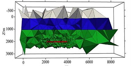
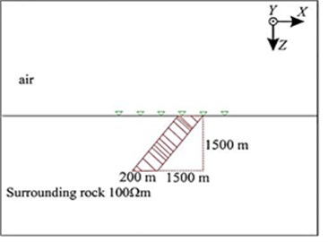
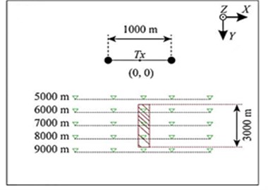
Fault fracture zones, contact zones and metal veins can often be approximated by inclined plates. Establish a three-dimensional land model as shown in Fig. 11: the air resistivity is 108 Ωm, and there is an angle in the uniform half-space model with the resistivity of 100 Ωm.

A 45° inclined plate-shaped body, with the top exposed on the ground, with a resistivity of 30 Ωm. The three-dimensional scale of the plate-shaped body is 200 m×3000 m×1500 m, and the distribution range along the $X$ direction: the width is 200 m, the top is [750, 950] m, and the bottom it is [–950, –750] m; along the $Y$ direction, the distribution range is [5500, 8500] m, and the length is 3000 m. On the ground ( $Z =$ 0 m), $Y =$ 5 km, 6 km, 7 km, 8 km, 9 km are arranged respectively. There are 205 measuring points in total, each measuring line is 2 km in length, containing 41 measuring points, and the interval is 50 m. The length of the grounding long wire source is 1km, and the center is placed at (0, 0, 0), along $X$ placed in the direction, the emission current is 1 A, and the emission frequency is sampled at logarithmic intervals between –1 and 1000 Hz, with a total of 11 sampling points [33, 34].

Fig. 11Land model of inclined plate

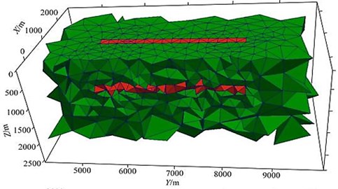
a)

b)

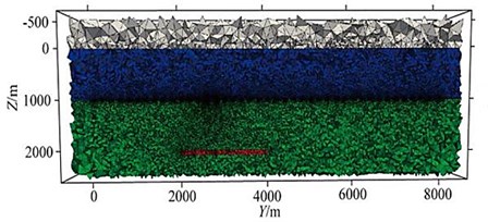
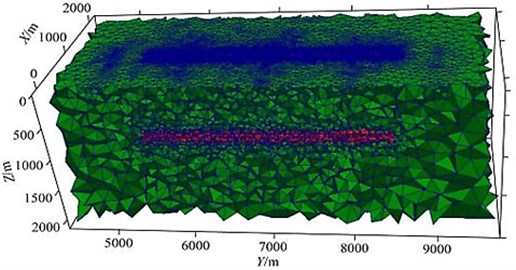
The calculation area of this example is 60 km×60 km×60 km, and the area of interest in the grid is extracted and displayed separately as shown in Fig. 12 (0 km $< X <$ 2 km, 4.5 km $< Y <$ 9.5 km, 0 km $< Z <$ 2 km). The mesh section is shown in Fig. 12(a). After 10 iterations, it converges (take 10 Hz as an example). At this time, the mesh has little effect on the change of the result. The final mesh section is shown in Fig. 12(b). There is good encryption everywhere.

Fig. 12Part grid diagram (land model)

a)

b)

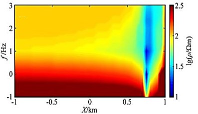
Fig. 13 shows the apparent resistivity slice of Kania.

Fig. 13Carnia apparent resistivity 3D slice

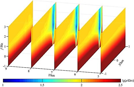
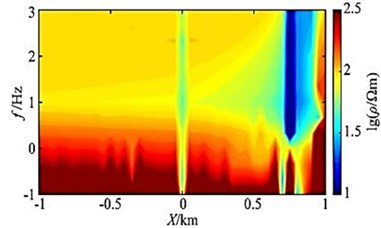
No oblique plate anomaly can be seen on the 5 km and 9 km survey lines, and it can be clearly seen on the 6 km, 7 km and 8 km survey lines. Low resistance is abnormal. The apparent resistivity profiles of the three slices are basically the same. At 750-950 m of the exposed surface area, due to the influence of static effects, there is a phenomenon of noodles in the apparent resistivity, and further inversion is needed to better determine the tilt the inclination of the slab body, and a clearer resistivity interface can still be seen between -750 and 750 m. This part of the abnormality is the influence of the inclined slab body. In order to verify the correctness of the results, especially the high frequency in the case of the results, we compared the profile with the 2D adaptive finite element algorithm at the 7 km survey line, and the results are basically the same, as shown in Fig. 14.

Fig. 14Y= 7 km slice of apparent resistivity of the line of measurement

a)

b)

In the high frequency band (100-1000 Hz), within the range of [-1 km, 0] the apparent resistivity is all 100 Ωm, thus verifying the correctness of the high-frequency results. On the apparent resistivity slice, we can see a more obvious oblique plate-like body abnormality, and there is a phenomenon of noodles at 750-950 m. However, the 2D slice reflects the infinitely extending sloping plate-shaped body in the $Y$ direction, the apparent resistivity is low and the abnormal value is lower, and there is a large calculation error near the source due to the influence of the algorithm.

5. Conclusions

This article uses an adaptive vector finite element algorithm is used to realize the CSEM3D forward simulation and the primary/secondary field separation algorithms are utilized for the calculation of the electromagnetic vibration spectrum field response. The adaptive mesh refinement algorithm based on posterior error estimation refines the mesh, reduce the singularity of the source point, and improve the numerical accuracy of the electromagnetic vibration spectrum field near the field source and the receiving point. High-quality finite element solution is obtained using unstructured tetrahedral element grid method for discretization of geoelectric model, while posterior error estimation method is used to guide the grid encryption. The algorithms utilized can calculate the electromagnetic vibration spectrum field of a galvanic source with a finite length in any posture, and the source and receiving points can be placed in any position, which has good versatility.

This article establishes a layered oil and gas model and the analytical solutions are compared and the relative error of horizontal electromagnetic vibration spectrum field component amplitude is observed less than 1 % and the phase difference of 1° is observed. It is revealed from the numerical simulation and analysis that for the vertical electromagnetic vibration spectrum field component, when the transmission and reception distance is small (less than 5 km), the amplitude the relative error is less than 1 %, and the phase difference is within 1°. However, when the transmission distance is greater than 5 km, the relative amplitude error is larger, and the maximum phase difference of the $E_{Z}$ component is 1.4. this experimentation verifies the correctness and accuracy of the algorithm.

The correctness of the proposed algorithm is further verified by establishing a horizontal thin plate-shaped high-resistance oil and gas reservoir model. The three-dimensional forward modelling algorithm of ocean controllable source electromagnetic vibration spectrum based on staggered grid finite volume discretization are compared and it was analysed that the amplitude and phase coincide very well. It was found that the effective anomaly can better reflect the high-resistance oil and gas compared to the amplitude curve. For the established land model, the apparent resistivity of the 5 survey lines is calculated. It was revealed from the outcomes that there is an obvious static effect at the surface outcrop, and further inversion is needed to better determine the position and inclination angle of the inclined plate.

References

R. Peng, B. Han, and X. Hu, “Exploration of seafloor massive sulfide deposits with fixed-offset marine controlled source electromagnetic method: numerical simulations and the effects of electrical anisotropy,” Minerals, Vol. 10, No. 5, p. 457, 2020, https://doi.org/10.3390/min10050457

Publisher
Y. Liu, Q. Sun, A. Sharma, A. Sharma, and G. Dhiman, “Line monitoring and identification based on roadmap towards edge computing,” Wireless Personal Communications, 2021, https://doi.org/10.1007/s11277-021-08272-y

Publisher
M. Fan and A. Sharma, “Design and implementation of construction cost prediction model based on SVM and LSSVM in industries 4.0,” International Journal of Intelligent Computing and Cybernetics, Vol. 14, No. 2, pp. 145–157, 2021, https://doi.org/10.1108/ijicc-10-2020-0142

Publisher
S. C. L. Freitas, L. C. O. Oliveira, P. S. Oliveira, B. Exposto, J. G. O. Pinto, and J. L. Afonso, “Modeling, design, and experimental test of a zero‐sequence current electromagnetic suppressor,” International Transactions on Electrical Energy Systems, Vol. 30, No. 2, 2020, https://doi.org/10.1002/2050-7038.12222

Publisher
I. V. Bochkarev and I. V. Bryakin, “Development of a new method of diagnostics electromagnetic drive power and commutation mechanisms,” Power Engineering: Research, Equipment, Technology, Vol. 22, No. 3, pp. 68–77, 2020, https://doi.org/10.30724/1998-9903-2020-22-3-68-77

Publisher
P. Lipinski and M. Leplawy, “WiFi electromagnetic field modelling for indoor localization,” Open Physics, Vol. 17, No. 1, pp. 352–357, 2019, https://doi.org/10.1515/phys-2019-0039

Publisher
“Evaluation of Electric and Magnetic Fields Distribution and SAR with the Help of Intensity of Time Averaged Electromagnetic Wave,” International Journal of Recent Technology and Engineering 2, Vol. 8, No. 2, pp. 5495–9498, 2019, https://doi.org/10.35940/ijrte.b2631.078219

Publisher
S. Hasan, N. Gurung, K. M. Muttaqi, and S. Kamalasadan, “Electromagnetic field-based control of distributed generator units to mitigate motor starting voltage dips in power grids,” IEEE Transactions on Applied Superconductivity, Vol. 29, No. 2, pp. 1–4, 2019, https://doi.org/10.1109/tasc.2019.2895468

Publisher
N. Afrin, F. Yang, J. Lu, and M. Islam, “Impact of induction motor load on the dynamic voltage stability of microgrid,” in 2018 Australian & New Zealand Control Conference (ANZCC), 2018, https://doi.org/10.1109/anzcc.2018.8606599

Publisher
D. R. Medina, E. Rappold, O. Sanchez, X. Luo, S. Rivera, D. Wu, and J. Jiang, “Fast assessment of frequency response of cold load pickup in power system restoration,” in 2016 IEEE Power and Energy Society General Meeting (PESGM), 2016, https://doi.org/10.1109/pesgm.2016.7741081

Publisher
A. Al-Nujaimi, M. A. Abido, and M. Al-Muhaini, “Distribution power system reliability assessment considering cold load pickup events,” IEEE Transactions on Power Systems, Vol. 33, No. 4, pp. 4197–4206, 2018, https://doi.org/10.1109/tpwrs.2018.2791807

Publisher
M. Kumar, O. V. Kulkarni, A. S. Vijay, and S. Doolla, “Investigation of induction motor support in weak microgrids using virtual synchronous generator,” in 2017 National Power Electronics Conference (NPEC), 2017, https://doi.org/10.1109/npec.2017.8310461

Publisher
C. Li, X. Wang, J. Gong, C. Ping, J. Guo, H. Guo, and Z. Wang, “Impacts of instantaneous heavy load on DC distribution network and their solution,” in 2020 IEEE/IAS Industrial and Commercial Power System Asia (I&CPS Asia), 2020, https://doi.org/.1109/icpsasia48933.2020.9208454

Publisher
A. Vandermeulen, T. Natali, T. Dionise, G. Paradiso, and K. Ameele, “Exploring new and conventional starting methods of large medium voltage induction motors on limited KVA sources,” in 2018 IEEE Industry Applications Society Annual Meeting (IAS), 2018, https://doi.org/10.1109/ias.2018.8544648

Publisher
S. F. Rabbi, J. T. Kahnamouei, X. Liang, and J. Yang, “Shaft failure analysis in soft-starter fed electrical submersible pump systems,” IEEE Open Journal of Industry Applications, Vol. 1, pp. 1–10, 2020, https://doi.org/10.1109/ojia.2019.2956987

Publisher
D. Penkov and C. Gaudeaux, “Mv motors starting with auto-transformer,” 2018 Petroleum and Chemical Industry Conference Europe (PCIC Europe), 2018, https://doi.org/10.23919/pciceurope.2018.8491415

Publisher
B. Q. Khanh, “On optimally positioning a multiple of dynamic voltage restorers in distribution system for global voltage sag mitigation,” in 2019 IEEE Asia Power and Energy Engineering Conference (APEEC), 2019, https://doi.org/10.1109/apeec.2019.8720695

Publisher
J. Chao, M. Huang, and A. Radzhabov, “Charged pion condensation in anti-parallel electromagnetic fields and nonzero isospin density,” Chinese Physics C, Vol. 44, No. 3, p. 034105, 2020, https://doi.org/10.1088/1674-1137/44/3/034105

Publisher
“Electromagnetic Spectrum,” Field Guide to Infrared Systems, pp. 1–1, 2019.

Search CrossRef
Z. Liu, Y. Zhang, A. Li, M. Xie, W. Bin, and C. He, “Development of a shear horizontal wave electromagnetic acoustic transducer with periodic grating coil,” International Journal of Applied Electromagnetics and Mechanics, Vol. 60, No. 4, pp. 545–563, 2019, https://doi.org/10.3233/jae-180120

Publisher
M. Poongodi, A. Sharma, M. Hamdi, M. Maode, and N. Chilamkurti, “Smart healthcare in smart cities: wireless patient monitoring system using IoT,” The Journal of Supercomputing, 2021, https://doi.org/10.1007/s11227-021-03765-w

Publisher
X. Xu, L. Li, and A. Sharma, “Controlling messy errors in virtual reconstruction of random sports image capture points for complex systems,” International Journal of System Assurance Engineering and Management, p. 1-8, 2021, https://doi.org/10.1007/s13198-021-01094-y

Publisher
G. K. Sodhi, S. Kaur, G. S. Gaba, L. Kansal, A. Sharma, and G. Dhiman, “COVID-19: Role of robotics, artificial intelligence, and machine learning during pandemic,” Current Medical Imaging Formerly: Current Medical Imaging Reviews, Vol. 17, 2021, https://doi.org/10.2174/1573405617666210224115722

Publisher
A. Ö. Özer and K. A. Morris, “Modeling and stabilization of current-controlled piezo-electric beams with dynamic electromagnetic field,” ESAIM: Control, Optimisation and Calculus of Variations, Vol. 26, p. 8, 2020, https://doi.org/10.1051/cocv/2019004

Publisher
P. Zradziński, J. Karpowicz, K. Gryz, L. Morzyński, R. Młyński, A. Swidziński, K. Godziszewski, and V. Ramos, “Modelling the Influence of Electromagnetic Field on the User of a Wearable IoT Device Used in a WSN for Monitoring and Reducing Hazards in the Work Environment,” Sensors, Vol. 20, No. 24, p. 7131, 2020, https://doi.org/10.3390/s20247131

Publisher
H. Cang, A. Labno, C. Lu, X. Yin, M. Liu, C. Gladden, Y. Liu, and X. Zhang, “Probing the electromagnetic field of a 15-nanometre hotspot by single molecule imaging,” Nature, Vol. 469, No. 7330, pp. 385–388, 2011, https://doi.org/10.1038/nature09698

Publisher
B. L. J. Gysen, K. J. Meessen, J. J. H. Paulides, and E. A. Lomonova, “General formulation of the electromagnetic field distribution in machines and devices using Fourier analysis,” IEEE Transactions on Magnetics, Vol. 46, No. 1, pp. 39–52, 2010, https://doi.org/10.1109/tmag.2009.2027598

Publisher
X. Tu and M. S. Zhdanov, “Robust synthetic aperture imaging of marine controlled-source electromagnetic data,” IEEE Transactions on Geoscience and Remote Sensing, Vol. 58, No. 8, pp. 5527–5539, 2020, https://doi.org/10.1109/tgrs.2020.2966727

Publisher
O. Sharabura and D. Kuryliak, “Electromagnetic field of the circular magnetic source in biconical section,” Information extraction and processing, Vol. 2020, No. 48, pp. 5–10, 2020, https://doi.org/10.15407/vidbir2020.48.005

Publisher
Y. Liu, “Application of perfectly matched layers in 3D transient controlled-source electromagnetic modeling by the rapid expansion method,” Geophysics, Vol. 85, No. 1, 2020, https://doi.org/10.1190/geo2018-0753.1

Publisher
D. Blatter, K. Key, A. Ray, C. Gustafson, and R. Evans, “Bayesian joint inversion of controlled source electromagnetic and magnetotelluric data to image freshwater aquifer offshore New Jersey,” Geophysical Journal International, Vol. 218, No. 3, pp. 1822–1837, 2019, https://doi.org/10.1093/gji/ggz253

Publisher
C. Qiu, S. Güttel, X. Ren, C. Yin, Y. Liu, B. Zhang, and G. Egbert, “A block rational Krylov method for 3-D time-domain marine controlled-source electromagnetic modelling,” Geophysical Journal International, Vol. 218, No. 1, pp. 100–114, 2019, https://doi.org/10.1093/gji/ggz129

Publisher
P. E. Tereshchenko, “Estimating the effective conductivity of the underlying surface based on the results of receiving the electromagnetic fields in the middle zone of an active source in the earth–ionosphere waveguide,” Seismic Instruments, Vol. 56, No. 5, pp. 578–583, 2020, https://doi.org/10.3103/s0747923920050126

Publisher
V. Y. Abramov, “Some peculiarities of the polarization structure of the electromagnetic field at high frequencies in geological sections: mathematical solutions and experiments,” RUDN Journal of Engineering Researches, Vol. 21, No. 2, pp. 123–130, 2020, https://doi.org/10.22363/2312-8143-2020-21-2-123-130

Publisher

About this article

Received

25 April 2021

Accepted

20 May 2021

Published

30 September 2021

DOI

https://doi.org/10.21595/jve.2021.22031

Keywords

controllable source electromagnetic vibration spectrum

three-dimensional performance

adaptive vector finites

unstructured mesh

Acknowledgements

Project of National Natural Science Foundation of China in 2017 Nonlinear modeling and predistortion linearization of MRI power amplifier with variable pulse excitation. Project No. 61701262.

Key scientific and technological projects in Henan Province Research on Application of Internet of vehicles technology based on video recognition in bus overload control. Project No. 182102310760.

The special project of Nanyang Normal University for doctors Simulation design and optimization of permanent magnet for small MRI system. Project No. ZX2016011.

This is an open access article distributed under the Creative Commons Attribution License, which permits unrestricted use, distribution, and reproduction in any medium, provided the original work is properly cited.

Previous article in issue Previous Next article in issue Next

Research article

2022 04 21

The response suppression method of electromagnetic vibration exciters based on the compensation current

Wei Li, Jun Cui, Junning Cui, Zhisheng Wang, Limin Zou

Research article

2022 01 25

Three-dimensional numerical simulation of multi-physical coupled environment during electromagnetic propulsion

Yuxin Yang, Peng Liu, Haojie Li, He Zhang

Research article

2020 02 15

Thermoelastic vibration analysis of disc brake based on multi-physical field coupling method

Sen Zhang, Jian Zhang

Research article

2019 02 15

Research of multi-point adaptive control strategy based on electromagnetic active vibration absorber

Weipeng Gao, Guo He, Shuyong Liu

Y. Cheng, M. Su, M. Hui, W. Liu, and Y. Zheng, “Mathematical simulation of adaptive vector finite element method for the analysis of electromagnetic vibration spectrum field response,” Journal of Vibroengineering, Vol. 23, No. 6, pp. 1332–1349, Sep. 2021, https://doi.org/10.21595/jve.2021.22031

Copy Extrica

Copied to clipboard!

TY  - JOUR
DO  - 10.21595/jve.2021.22031
UR  - https://doi.org/10.21595/jve.2021.22031
TI  - Mathematical simulation of adaptive vector finite element method for the analysis of electromagnetic vibration spectrum field response
T2  - Journal of Vibroengineering
AU  - Cheng, Yiyuan
AU  - Su, Mingyang
AU  - Hui, Ming
AU  - Liu, Wei
AU  - Zheng, Yangbing
PY  - 2021
DA  - 2021/09/30
PB  - JVE International Ltd.
SP  - 1332-1349
IS  - 6
VL  - 23
SN  - 1392-8716
SN  - 2538-8460
ER  - 

Copy Ris

Copied to clipboard!

@article{Cheng_2021,
	doi = {10.21595/jve.2021.22031},
	url = {https://doi.org/10.21595/jve.2021.22031},
	year = 2021,
	month = {sep},
	publisher = {{JVE} International Ltd.},
	volume = {23},
	number = {6},
	pages = {1332--1349},
	author = {Yiyuan Cheng and Mingyang Su and Ming Hui and Wei Liu and Yangbing Zheng},
	title = {Mathematical simulation of adaptive vector finite element method for the analysis of electromagnetic vibration spectrum field response},
	journal = {Journal of Vibroengineering}
}

Copy Bibtex

Copied to clipboard!

[1]Y. Cheng, M. Su, M. Hui, W. Liu, and Y. Zheng, “Mathematical simulation of adaptive vector finite element method for the analysis of electromagnetic vibration spectrum field response,” Journal of Vibroengineering, vol. 23, no. 6, pp. 1332–1349, Sep. 2021, doi: 10.21595/jve.2021.22031.

Copy IEEE

Copied to clipboard!

Cheng, Yiyuan, Mingyang Su, Ming Hui, Wei Liu, and Yangbing Zheng. “Mathematical Simulation of Adaptive Vector Finite Element Method for the Analysis of Electromagnetic Vibration Spectrum Field Response.” Journal of Vibroengineering 23, no. 6 (September 30, 2021): 1332–49. https://doi.org/10.21595/jve.2021.22031.

Copy Chicago

Copied to clipboard!

Mathematical simulation of adaptive vector finite element method for the analysis of electromagnetic vibration spectrum field response

Abstract

Highlights

1. Introduction

2. Unstructured grid vector finite element method

2.1. Governing equation

2.2. Finite element analysis

3. Adaptive mesh refinement algorithm based on posterior error estimation

4. Results and analysis of the numerical calculation

4.1. One-dimensional oil and gas model

4.2. Three-dimensional oil and gas model

4.3. Three-dimensional tilt anomaly model

5. Conclusions

References

About this article

Related Articles