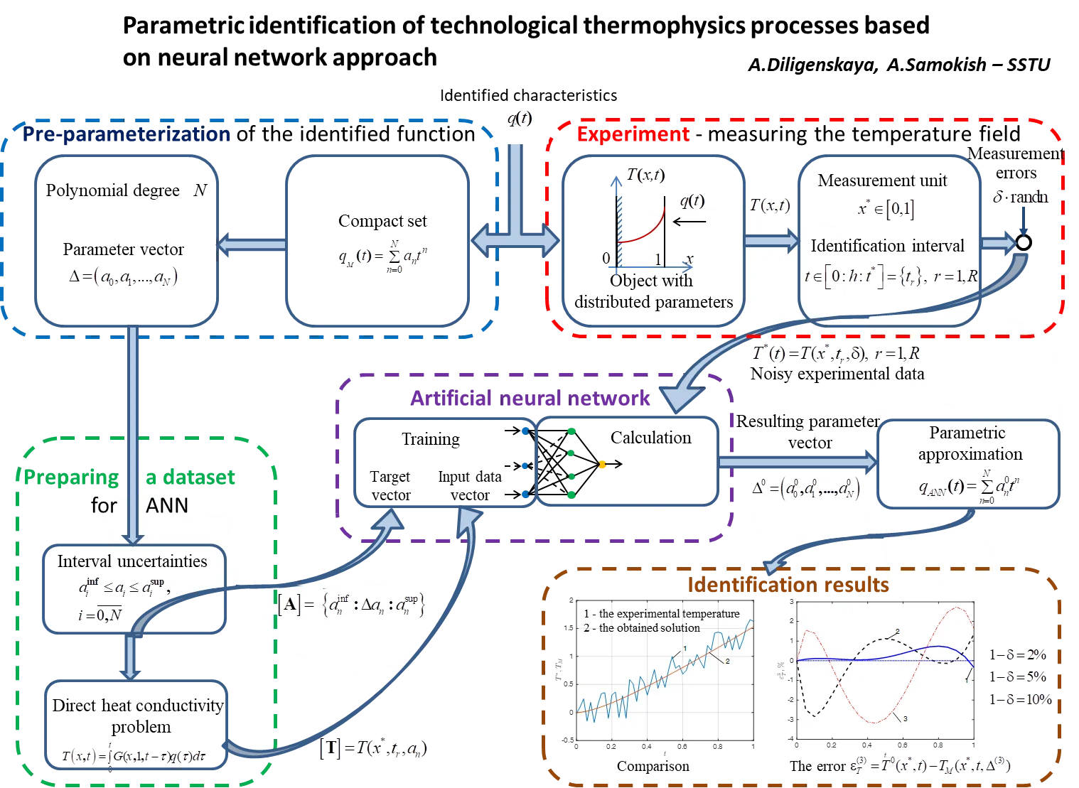
Abstract
In this paper, the inverse problem of technological thermophysics under the influence of disturbing factors is under study. In the problem of identifying the process of nonstationary heat conduction, it is required to concretize its mathematical model by qualitatively and quantitatively expressing an unknown characteristic based on the results of experimental studies. It is necessary to determine the uncontrolled time-varying heat flux density on the surface of the heated product from the noisy temperature measurement results at a certain point inside the object. The problem is formulated in an extreme setting as a problem of optimal control of an object with distributed parameters, in which the quadratic value of the temperature discrepancy between experimental and model data is used as an optimality criterion. The preliminary parametrization of the desired control on a compact set of polynomial functions implements the reduction to the parametric optimization problem. Physically substantiated solutions to inverse heat conduction problems are found as a result of their sequential parametric optimization using an algorithmically accurate method based on optimal control theory. The proposed solution combines the advantages of an accurate analytical method, which allows taking into account the physical essence of the process of interest and artificial intelligence methods, which provide great opportunities to find an quasioptimal solution under conditions of uncertainty in the mathematical description of the process. The analytical method of sequential parameterization provides a search for solutions on a compact set of smooth functions, as a result of which there is a reduction to the problem of parametric optimization. Measurement errors lead to processing large amounts of data, which necessitates the use of artificial neural networks for parametric optimization of the identified characteristics. The attained results confirm the possibility of obtaining adequate solutions to the inverse problems of thermal conductivity with the intensity of the measurement noise in the range of 0-15 %. In the investigated class of solutions, with a suitable setting of the ranges of belonging of the parameters, the error in approximating the temperature state can be up to 2-5 %, and the error in restoring the unknown characteristic can be up to 7-10 %.
Highlights
- The inverse problem of technological thermophysics, in which it is required to determine the time-varying heat flux density based on the perturbed temperature measurement results, is under study.
- A problem of optimal control of an object with distributed parameters is formulated. Physically substantiated solutions are found as a result of sequential parametric optimization of the desired control on a compact set of polynomial functions.
- On the basis of an exact mathematical model of the heat conduction process, a parametric optimization problem is formulated. An artificial neural network is used to solve it under the influence of disturbing factors.
- The values of the coefficients of the parametric representation of the desired characteristic, taking into account their interval uncertainties, form the target vector. The corresponding set of solutions to direct heat conduction problems forms the input data of the neural network.
1. Introduction
This work is devoted to the search for methods for solving inverse problems, formulated in relation to equations of mathematical physics of parabolic type and providing for the definition of an unknown function that sets the boundary conditions when the input data are not fully known. Objects described by equations of this class are characterized by the spatial distribution of the modeled state function, and in some cases, input quantities, and refer to the systems with distributed parameters. Mathematical models based on differential equations in partial derivatives of parabolic type are widely used in many industrial technologies to describe the processes of unsteady heat conduction, heat and mass transfer, unsteady diffusion, electromagnetic waves propagation, and others.
The main difficulty in solving inverse problems of mathematical physics (IPMP) is their belonging to the class of ill-posed problems, which necessitates the use of special numerical regularizing algorithms to obtain a stable solution [1], [2]. In the case of an unavoidable measurement error or other disturbances, the problem of constructing special regularizing algorithms for a stable solution of such problems becomes especially urgent [3], [4].
In the theory of inverse ill-posed problems of mathematical physics, a large number of methods and computational algorithms have been developed that make it possible to obtain regular solutions based, as a rule, on the use of smoothing functionals or additional restrictions on the class of sought solutions [5]-[7]. These approaches require significant computational efforts, depending on factors that are difficult to formalize [1], [2] or the availability of a priori information about the solution, which is usually absent [1], [4]. In such a situation, the development of methods for solving inverse and ill-posed problems of mathematical physics is an urgent problem. It makes possible to obtain stable solutions with satisfactory accuracy while reducing the computational complexity of methods and algorithms.
In the papers [8]-[11], the authors propose an analytical method of parametric optimization, which searches for solutions in the class of physically realizable functions based on their smoothness. The advantages of this approach are an accurate mathematical model that takes into account the qualitative physical laws and basic properties of the process under study, as well as displaying the solution in an analytical form, which provides benefits for its subsequent use in solving technological problems of various directions (control, monitoring, control, forecasting, diagnostics process and other tasks). The disadvantage of the approach may be its limited application under conditions of inevitable disturbing factors due to the sensitivity of the developed method, which uses analytical optimality conditions, to the level of input data error.
This paper presents an approach to the search for physically grounded solutions of the IPMP using the example of parabolic equations on compact sets of polynomial functions under the conditions of disturbed input data based on parametric optimization implemented using artificial neural networks (ANN). The solution to the problem is obtained on the basis of a combination of an accurate analytical approach, which takes into account information about the physical characteristics of processes and systems with distributed parameters, and intelligent technologies that allow finding the quasioptimal solution under conditions of uncertainty in the mathematical description of the process.
The proposed approach allows us to find solutions to inverse problems without the use of laborious numerical regularizing algorithms that depend on factors that are difficult to formalize on a compact set of smooth functions, taking into account the measurement noise acting over a sufficiently wide range, with an accuracy acceptable for practical applications. Difficulties associated with the need to process a large amount of input information affect the training of an artificial neural network, and practically do not affect its performance when it is subsequently used to solve a specific problem of identifying the boundary conditions of the process.
2. Formulation of the problem
We consider a linear one-dimensional homogeneous partial differential equation of parabolic type, given in relative coordinates:
supplemented by initial and boundary conditions of the second kind:
The formulation of the inverse problem provides for the presence of input information , where in most real cases the value of the state function is used – temperature , – obtained as a result of its control (measurements) at some fixed point [0,1] at discrete moments in the identification interval and containing measurement errors . In the inverse boundary problem, it is required to determine the unknown time-dependent heat flux density , applied to the outer boundary 1, with the remaining parameters and characteristics of the object given.
As a rule, a modern approach to the formulation of inverse problems is their definition in a variational formulation, which provides for the minimization of the objective functional in the space of possible solutions [12]. As a measure of the correspondence of the mathematical model to the real process, the value of the temperature residual is used, written in a quadratic or uniform metric [12]-[14]. Then the inverse problem is considered as an optimal control problem in which the conditions for the extremum of the formulated target functional of the temperature residual are investigated [14].
In this paper the inverse problem is formulated in a variational setting as an optimal control problem, where, based on the experimental data obtained under the conditions of disturbances, it is necessary to restore the unknown characteristic , minimizing the deviation between the experimental results and the values of the state function , calculated on the basis of the mathematical model (Eq. (1)-(2)) when using found solution on a given identification interval at the same point . To estimate the deviation of the model temperature from the experimental one, a functional based on the squared error is used:
where the function to be identified is considered as the desired control and is subject to the conditions of belonging to the corresponding set . Quadratic error functional Eq. (3) is chosen as the most widespread in neural network technologies, which are used further in solving the problem of parametric optimization.
3. Parametric optimization of the desired characteristic
To solve the formulated problem (Eq. (3)), a transition is made from the original set to the class of functions physically substantiated in the process of identifying functions that form a compact set. As physically realizable characteristics specified on the basis of requirements for their smoothness, we consider a set of polynomial functions of the form:
where the exact value ensures that the identified characteristic belongs to a specific class of functions. Thus, the value and the corresponding vector of parameters uniquely determine the parametric representation according to Eq. (4) of the sought-for heat flux density .
Then the mathematical description of the process under study (Eq. (1)-(2)) makes it possible to obtain the calculated value of the state function as a reaction to the boundary effect , expressed in parametric form, at given values and , which corresponds to the temperature parameterization procedure. The resulting representation leads to the parametric optimization problem:
with respect to the desired vector of parameters .
Thus, the narrowing of the original class of solutions to a compact set of polynomial functions according to Eq. (4) given by the number and the corresponding vector , allows us to formulate the parametric optimization problem given in a form of Eq. (5), and thus corresponds to the transition from the original ill-posed problem to the conditionally correct formulation, which solution does not require the use of regularization methods.
Proposed approach to identifying an unknown function is based on constructing a sequence of functions on a compact set , that minimizes the quadratic deviation with increasing number and, thus, converges to the exact solution . Based on the Weierstrass theorem [15], the solutions obtained are regular. Each successive approximation of the sequence can be considered as an intermediate solution, and the computational procedure can be stopped when the deviation of the calculated value from the measured one meets the requirements of a given accuracy.
At a low level of perturbations, the solution to the problem can be realized using the minimax optimization method [8]-[11], based on the analytical optimality conditions [16]. In a situation where the input data is significantly distorted by measurement errors, it is proposed to solve the problem using artificial intelligence methods that allow processing large data arrays to find vector values , that ensure the fulfillment of the quadratic optimality criterion Eq. (5).
4. Construction of neural networks for solving inverse problems of mathematical physics
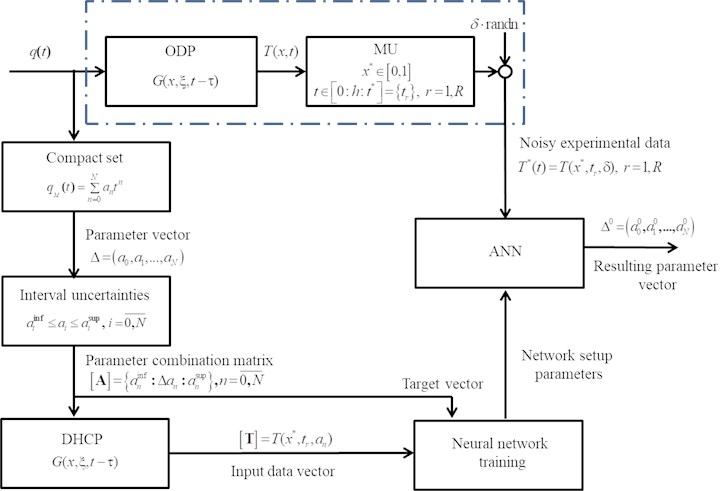
There are no general solution methods that allow one to find the global extremum of functional Eq. (5) under the conditions of the action of perturbations. When using input data , that take into account measurement errors , the method of sequential parameterization [8]-[11], which is successfully used to find solutions to inverse problems of heat conduction under deterministic influences, is proposed to be supplemented with the use of ANN. Neural networks are profitably applied to solve problems of approximating time series, constructing dynamic dependencies, predicting the values of functions at future moments in time related to direct problems [17]-[19]. By choosing the type of neural network, the number of layers and neurons in each of the layers, setting the activation function and the network learning algorithm, the behavior of the state function is reproduced with a sufficient degree of accuracy. To search for solutions to problems in mathematical physics, it is recommended to use such neural networks as multilayer perceptron, networks with radial basis functions, probabilistic networks, generalized regression networks [20], [21]. Neural network technologies can also be used to solve inverse problems [22]-[24].
The formulated parametric optimization problem (Eq. (5)) is considered under conditions of interval uncertainties, when the amount of a priori information about the values of the parameters is limited by information about the boundaries of the interval of their possible change:
A set of possible combinations of parameters , forms a ensemble of temperature curves , , that satisfy the conditions (Eq. (6)). Then the problem (Eq. (5)) is considered with respect to a set of temperature realizations that satisfy all possible combinations of parameter values , . To solve this problem, neural networks are used that allow processing large data arrays containing possible values of the parameters of the identified characteristic and the corresponding realizations of the temperature field.
Solution to the problem (Eq. (5)) based on noisy input data is reduced to a step-by-step search for the values of the parameter vector for increasing values . The iterative procedure ends at , when the solution obtained at the next step ensures the achievement of an absolute or relative accuracy.
At each iteration, for a chosen number and a given, thus, the structure of the vector , the problem of parametric optimization (Eq. (5)) taking into account the perturbed input data is reduced to the execution of the following algorithm.
1) Based on a priori information about design, technological or other constraints, the permissible range of variation of the desired characteristic is determined , and then the approximate boundaries of possible intervals of change in values are determined of every parameter , . For each of the them, a sampling step is selected and a one-dimensional array of discrete parameter values is formed each with the dimension , .
2) Based on one-dimensional vectors an array of sample values of all parameters is formed, i.e. a matrix is drawn up , with the dimension , containing a set of all possible combinations of discrete parameter values from the corresponding ranges of their variation. Thus, each row of the matrix contains some variant of the admissible realizations of the combination of discrete values , of the vector , , and the complete matrix consists of all possible combinations. The matrix composed in this way forms the target vector in the development of the ANN.
3) On the basis of the mathematical model of an object with distributed parameters (Eq. (1)-(2)), a set of direct problems of heat conduction is solved for all variants of combinations of parameters from the matrix on a given identification interval . As a result, each -th row of matrix is associated with a model temperature realization , obtained at discrete times of the identification interval for each variant of the combination of parameters , , .
4) A neural network model of the inverse problem of heat conduction is created. The input data of the ANN is the set of all temperature realizations , , and the target values are the corresponding parameters that form the matrix . The neural network training procedure consists in calculating the weight coefficients (synaptic weights) that minimize the deviation error between the temperature realizations obtained on the basis of the neural network model , that correspond to the found solutions Δ ANN, and the specified temperature realizations for the entire data array .
The ANN constructed in this way is used further to calculate on the basis of noisy experimental data , obtained at the temperature control point [0, 1] in the identification interval ; 0, the parameter values, providing the best coincidence of the calculated data and measurement results according to the criterion of the minimum squared error. The obtained solution to the parametric optimization problem (Eq. (5)), corresponding to the conditionally correct formulation of the inverse heat conductivity problem, belongs to a compact set of functions of a given form Eq. (4) and is stable, regardless of the input data error. The magnitude of the error only affects the accuracy of the reconstruction of the identified characteristic. The block diagram reflecting the procedure for solving the inverse problem of technological thermophysics is shown in Fig. 1.
Fig. 1Solution pattern to the inverse heat conductivity problem: ODP – object with distributed parameters, MU – measurement unit, DHCP – direct heat conductivity problem
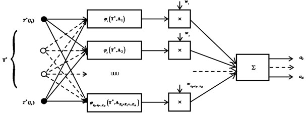
The formulated parametric optimization problem (Eq. (5)) was solved using radial basis function network (RBFN) [20], [21], which showed efficiency in solving direct problems of mathematical physics. These structures contain an inner layer consisting of radial elements that implement the Gaussian function, and a linear layer that provides a weighted average estimate. The weighting factors are obtained by minimizing the distance between the calculated values , corresponding to the found vector of parameters and the corresponding realizations of the input data array . A linear combination of the output signals of the radial elements for all elements of the training sample, with the found weight coefficients, makes it possible to obtain the resulting estimate of the values of the parameters of the polynomial representation according to Eq. (4) of the identified characteristic . A diagram showing the architecture of a radial basic neural network for solving a parametric optimization problem is shown in Fig. 2.
Fig. 2RBF – network architecture, φT*,A – radial basis functions, w – network setup parameters
5. Results and discussion
According to the described method, on the basis of the mathematical model (Eq. (1), (2)), the inverse boundary problem of heat conduction was solved by restoring the unknown function of the heat flux density:
using experimental data taking into account the additive measurement error , where – exact solution of the heat conduction problem (Eq. (1), (2)), and “randn” function simulates a normal distribution with zero mean value and standard deviation .
Temperature dependence was obtained at the point 0.9 based on the general solution of the heat problem, expressed in integral form:
where – Green’s function corresponding to the boundary value problem (Eq. (1), (2)). In accordance with Eq. (7), the flux density is taken to be , and Eq. (8) takes the form:
The parametric optimization problem was solved in the class of polynomial functions according to Eq. (4) with 2, 3. Temperature curves with 3 which are the input data for the ANN, are obtained on the basis of Eq. (8) when specifying in the form of a polynomial dependence (Eq. (4)) with 3, , which has the following form:
The case 2 can be considered as a special case 3 with 0.
The problem is solved using RBF – network on the identification interval with the following data 2, 2 taking into account measurement errors distributed according to the normal law with standard deviation 0-15 %.
Some results of solving the problem are presented in Figs. 3-6.
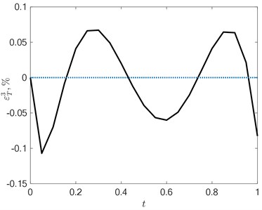
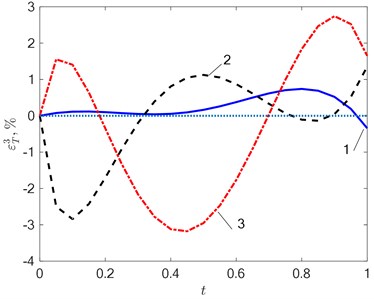
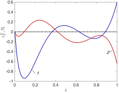
The figures show the change in the configuration of the temperature discrepancy with an increase in the intensity of the interference when searching for solutions in the class of functions 3. With no interference (Fig. 3(a)) alternating extrema are present on the curve – , and the error in approximating the temperature field is less than 1 %. With an increase in the level of measurement error, the curve of the temperature residual is distorted (Fig. 3(b)), which leads to an increase in the approximation error. A similar situation is when 2 and 3 (Fig. 4, 5). In the general case, the solution in the class of functions with the number 3 allows us to obtain greater accuracy than with 2 both for approximating the temperature (Fig. 4(a), 5(a)) and for identifying the unknown function – the heat flux density (Fig. 4(b), 5(b)), but in each case the results based on the analysis of random processes using neural networks may differ. At the same time, there is no unambiguous relationship between the error - and – as in most cases, this happens when using deterministic algorithms [8]-[11].
Fig. 3The error εT3=T0x*,t-TMx*,t,Δ3 in the approximation of the temperature field at N= 3 in a) the absence of interference (δ= 0 %) and b) its action 1-δ= 2 %; 2-δ= 5 %; 3-δ= 10 %
a)
b)
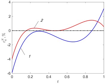
Fig. 4a) Error εTN=T0x*,t-TMx*,t,ΔN in approximating the temperature dependence and b) error εqN= q0t-qt,ΔN of reconstruction of the identified characteristic at δ= 2 %: 1 – N= 2; 2 – N= 3
a)
b)
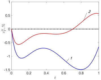
With an increase in the level of perturbation, the configuration of the temperature field error changes, which leads to a decrease in the accuracy of the temperature approximation and the identified function. This dependence has an ambiguous character for the restoration of both the state function and the desired characteristic. Artificial intelligence methods ensure the accuracy of solving the problem, acceptable for engineering calculations (Fig. 6), in the selected range of measurement error with a given input information.
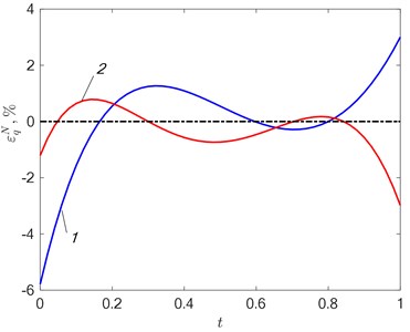
Fig. 5a) Fitting error εTN=T0x*,t-TMx*,t,ΔN and b) departure εqN=q0t-qt,ΔN in approximating the desired effect at δ= 15 %: 1 – N= 2; 2 – N= 3
a)
b)
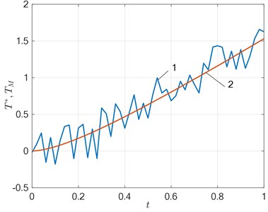
Fig. 6Comparison of the solution obtained with the experimental temperature 1 – T*t, δ= 15 %; 2 – TMx*,t,Δ3, N= 3
6. Conclusions
In this paper, using the example of the boundary value inverse problem of heat conduction, an approach to solving inverse problems of mathematical physics is presented, which combines the advantages of the exact analytical method, which is the basis for the identification of objects with distributed parameters on a compact set of polynomial functions, and artificial intelligence methods that allow processing large amounts of data and used for solving the problem of parametric optimization in conditions of perturbation of input information. The results obtained confirm the possibility of using neural networks in solving the problem of parametric optimization using the example of the inverse heat conductivity problem. The effectiveness of the results obtained depends on the level of measurement error and the specified values of the boundaries of the intervals of the probable change in the parameters.
To improve the accuracy of the solution, it is necessary to increase the degree of the approximating polynomial and, accordingly, the dimension of the sought vector of parameters , each of which , under data uncertainty is set on a certain admissible interval. With an increase of the number , the complexity and cumbersomeness of the neural network rapidly occurs. Moreover, some a priori information about the technological limitations of the device or process under study must be known for the adequate parameter setting.
The computational complexity of the proposed approach is associated with a large volume of processed data with an increase in the number of estimated parameters, which requires significant computing resources and time. These requirements are necessary only at the stage of training the neural network. The trained neural network is versatile and can be used repeatedly in the study of typical heat conduction processes.
References
-
O. M. Alifanov, International Series in Heat and Mass Transfer. Berlin, Heidelberg: Springer Berlin Heidelberg, 1994, https://doi.org/10.1007/978-3-642-76436-3
-
J. V. Beck, B. Blackwell, and C. R. St. Clair, “Inverse heat conduction. Ill-posed problems,” ZAMM – Journal of Applied Mathematics and Mechanics / Zeitschrift für Angewandte Mathematik und Mechanik, Vol. 67, No. 3, pp. 212–213, 1987, https://doi.org/10.1002/zamm.19870670331
-
A. N. Tikhonov and V. Ya Arsenin, Solutions of Ill-Posed Problems. Washington: John Wiley & Sons, 1977.
-
A. N. Tikhonov, A. V. Goncharsky, V. V. Stepanov, and A. G. Yagola, Regularizing Algorithms and a Priori Information. Moscow: Nauka, 1983.
-
M. N. Özisik and H. R. B. Orlande, Inverse Heat Transfer. Routledge, 2018, https://doi.org/10.1201/9780203749784
-
F. Yaman, V. G. Yakhno, and R. Potthast, “A survey on inverse problems for applied sciences,” Mathematical Problems in Engineering, Vol. 2013, pp. 1–19, 2013, https://doi.org/10.1155/2013/976837
-
R. Potthast, “A survey on sampling and probe methods for inverse problems,” Inverse Problems, Vol. 22, No. 2, pp. R1–R47, Apr. 2006, https://doi.org/10.1088/0266-5611/22/2/r01
-
A. N. Diligenskaya and Y. Rapoport, “Analytical methods of parametric optimization in inverse heat-conduction problems with internal heat release,” Journal of Engineering Physics and Thermophysics, Vol. 87, No. 5, pp. 1126–1134, Sep. 2014, https://doi.org/10.1007/s10891-014-1114-1
-
A. N. Diligenskaya and Y. Rapoport, “Method of minimax optimization in the coefficient inverse heat-conduction problem,” Journal of Engineering Physics and Thermophysics, Vol. 89, No. 4, pp. 1008–1013, Jul. 2016, https://doi.org/10.1007/s10891-016-1462-0
-
A. N. Diligenskaya, “Solution of the retrospective inverse heat conduction problem with parametric optimization,” High Temperature, Vol. 56, No. 3, pp. 382–388, May 2018, https://doi.org/10.1134/s0018151x18020050
-
A. Diligenskaya, “Methods of sequential parametric optimization in inverse problems of technological thermophysics,” in 2019 XXI International Conference Complex Systems: Control and Modeling Problems (CSCMP), pp. 267–270, Sep. 2019, https://doi.org/10.1109/cscmp45713.2019.8976763
-
O. M. Alifanov, E. A. Artyukhin, and S. V. Rumyantsev, Extreme Methods for Solving Ill-Posed Problems with Applications to Inverse Heat Transfer Problems. New York – Wallingford, U.K.: Begell House, 2015.
-
O. M. Alifanov, “The extremal formulations and methods of solving inverse heat conduction problems,” in Inverse Heat Transfer Problems, Berlin, Heidelberg: Springer Berlin Heidelberg, 1994, pp. 150–191, https://doi.org/10.1007/978-3-642-76436-3_7
-
Yu. M. Matsevity, Inverse Heat Conduction Problems, 1 vol. Methodology. Kyiv: Institute for Problems in Mechanical Engineering, National Academy of Sciences of Ukraine, 2008.
-
A. Pinkus, “Weierstrass and approximation theory,” Journal of Approximation Theory, Vol. 107, No. 1, pp. 1–66, Nov. 2000, https://doi.org/10.1006/jath.2000.3508
-
E. Ya. Rapoport, Alternance Method for Solving Applied Optimization Problems. (in Russian), Moscow: Nauka, 1986.
-
T. Kohonen, Springer Series in Information Sciences. Berlin, Heidelberg: Springer Berlin Heidelberg, 2001, https://doi.org/10.1007/978-3-642-56927-2
-
H. N. Mhaskar, “Neural networks for optimal approximation of smooth and analytic functions,” Neural Computation, Vol. 8, No. 1, pp. 164–177, Jan. 1996, https://doi.org/10.1162/neco.1996.8.1.164
-
D. Elbrächter, D. Perekrestenko, P. Grohs, and H. Bölcskei, “Deep neural network approximation theory,” arXiv:1901.02220, Mar. 2021.
-
M. D. Buhmann, Radial Basis Functions: Theory and Implementations. United Kingdom: Cambridge University Press, 2003.
-
P. V. Yee and S. Haykin, Regularized Radial Basis Function Networks: Theory and Applications. New York, John Wiley, 2001.
-
J. Krejsa, K. A. Woodbury, J. D. Ratliff, and M. Raudensky, “Assessment of strategies and potential for neural networks in the inverse heat conduction problem,” Inverse Problems in Engineering, Vol. 7, No. 3, pp. 197–213, Jun. 1999, https://doi.org/10.1080/174159799088027694
-
V. V. Berdnik and R. D. Mukhamedyarov, “Application of the method of neural networks to solution of the inverse problem of heat transfer,” High Temperature, Vol. 41, No. 6, pp. 839–843, Nov. 2003, https://doi.org/10.1023/b:hite.0000008342.42066.84
-
V. I. Gorbachenko and M. V. Zhukov, “Solving boundary value problems of mathematical physics using radial basis function networks,” Computational Mathematics and Mathematical Physics, Vol. 57, No. 1, pp. 145–155, Jan. 2017, https://doi.org/10.1134/s0965542517010079
About this article

This work was performed at the Samara State Technical University and supported by the Ministry of Science and Higher Education of the Russian Federation (basic part of a research project no. 0778-2020-0005).
