Dynamic simulation of nonlinear vibration on large horizontal axis turbine blades using a finite differential method

Zhu, You-Feng; Ren, Yong-Sheng; Dai, Qi-Yi

Journal of Vibroengineering

Browse Journal

Submit article

Published: 31 December 2013

Check for updates

Dynamic simulation of nonlinear vibration on large horizontal axis turbine blades using a finite differential method

You-Feng Zhu¹

Yong-Sheng Ren²

Qi-Yi Dai³

^{1, 2, 3}Shandong University of Science & Technology, Qingdao 266590, China

Cite the article Download PDF

Downloads 1126

Abstract

According to Kallesøe’s model of turbine blades, two methods were developed to solve the nonlinear vibration of blades, namely, nonlinear non-autonomous system with gravity effect and nonlinear autonomous system without gravity effect. The equations were changed into the mass and stiffness matrices using a finite difference method on the boundary conditions of cantilever beams. By the time discretion methods and the Matlab vibration toolboxes, the displacements and the phase tracks of blade tip were simulated in the directions of lead-lag, flapping and twisting. Then the amplitude-frequency and phase-frequency characteristic curves were plotted by the analysis of non-autonomous rotating turbine blades. Finally all simulation results were compared among the nonlinear system and the linear system. The nature frequencies and the convergence of the systems were also discussed.

1. Introduction

At present, the large wind turbine blade structure models contain crossed elastic hinge presented in [1] and continuous distribution parameters presented in [2, 3]. In 2007, Kallesøe introduced a new coordinate system of turbine blades based on Hodges-Dowell’s model, and established the dynamic equations presented in [4], but only studied on the linear parts of the blades. This paper has retained the nonlinear parts, to better study the lead-lag, flapping and twisting of turbine blades. The blades became into nonlinear non-autonomous systems with gravity effect and nonlinear autonomous systems without gravity effect using a finite difference method on the boundary conditions of cantilever beams, which can display the whole process of rotating blades, and have an engineering significance.

There are many methods, such as harmonic balance method presented in [5-8],perturbation method presented in [9, 10], Poincare method presented in [11, 12], average method, asymptotic method presented in [13-15], and the method of multiple scales presented in [16-17],to study the nonlinear vibration of large horizontal axis wind turbine blades. Scholars at home and abroad, have fall over each other to research the method of harmonic balance in these years. But this nonlinear solution exists limitation. For example, Galerkin algorithm as a harmonic balance method is based on the linear modality, which is obtained from the linear equations or directly from the empirical formula. So it is not accurate. Finite difference methods by dispersing the nonlinear system, as long as the increasing number of nodes, in theory is an exact solution, which also make simulation simpler in time domain, more convenient in frequency domain based on FFT. In addition, a finite difference method is particularly suitable for processing variable parameters along the blade geometric axis.

2. The model of wind turbine blades

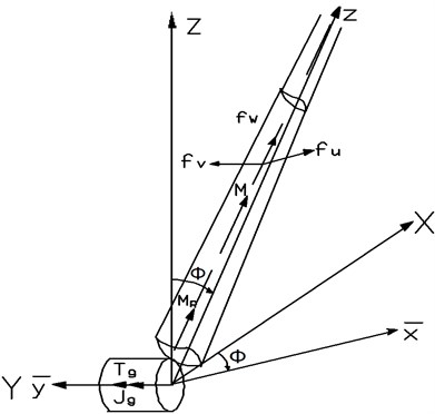
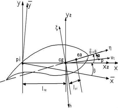
Kallesøe established a structure model of turbine blades in Fig. 1 presented in reference [3], on which coordinate transformation and the establishment of differential equation have been introduced. The finite differential method is more convenient in analysis of tapered cross section blades. The blades can be solid metal materials, also be a hollow composite material. Based on the equations in reference [3], retention of the first and second order Taylor quantity, neglecting higher-order quantity, considering gravity and ignoring the aerodynamic parameters, nonlinear motion equations in $x$ , $y$ , $z$ directions can be gained as follows in Formula (1), (2) and (3):

1

m \ddot{u} - Ω^{2} m (s (R - s) u^{'})^{'} + (E_{ξ} Ι_{ξ} {c o s}^{2} (θ) + E_{η} Ι η {s i n}^{2} (θ)) {u^{″}}^{″} + (E_{ξ} Ι_{ξ} - E_{η} Ι η) c o s (θ) s i n (θ) {v^{″}}^{″} - (E_{ξ} Ι_{ξ} - E_{η} Ι η) {(φ (u^{″} s i n (2 θ) - v^{″} c o s (2 θ)))}^{''} - Ω^{2} m c o s (β) (u c o s (β) - v s i n (β)) = - m g s i n (Ω t) c o s (β),

2

m \ddot{v} - Ω^{2} m s ((R - s) v^{'})^{'} + (E_{ξ} Ι_{ξ} {s i n}^{2} (θ) + E_{η} Ι η {c o s}^{2} (θ)) {v^{″}}^{″} + (E_{ξ} Ι_{ξ} - E_{η} Ι η) c o s (θ) s i n (θ) {u^{″}}^{″} + (E_{ξ} Ι_{ξ} - E_{η} Ι η) (φ {(u^{″} c o s (2 θ) + v^{″} s i n (2 θ))}^{''} + Ω^{2} m s i n (β) (u c o s (β) - v s i n (β)) = m g s i n (Ω t) s i n (β),

3

(I_{g} + m l_{c g}^{2}) \ddot{φ} - G J (φ^{'} + u^{″} v^{'})^{'} - E_{η} I_{η η ξ} (φ^{'} (u^{″} s i n (θ) - v^{″} c o s (θ))^{'} + E_{ξ} I_{η ξ ξ} (φ^{'} (u^{″} c o s (θ) - v^{″} s i n (θ))^{'} = m g l_{c g} s i n (Ω t) (s i n (θ + β) .

Fig. 1The model of a horizontal axis turbine blade

a)

b)

3. The establishment of general nonlinear equations

3.1. Finite difference discretization

Before finite difference discretization, the difference solution and curve fitting on the parameters of wind turbine blades must be done to get values in different nodes. The parameters in Formula (1), (2) and (3) are $m = m (s)$ , $θ = θ (s)$ , $Ι_{ζ} = Ι_{ζ} (s)$ , $Ι_{η} = Ι_{η (s)}$ , $C = C (s)$ . The boundary conditions of blades are as follows:

4

u (0, t) = u^{'} (0, t) = v (0, t) = v^{'} (0, t) = 0,

u^{″} (R, t) = v^{″} (R, t) = u^{‴} (R, t) = v^{‴} (R, t) = 0,

φ (0, t) = φ^{'} (0, t) = 0 .

The boundary conditions in $X$ and $Y$ directions are the same, so now fourth order derivative in $x$ -direction as an example is used to illustrate the difference discrete process. According to the Taylor expansion form, each derivative of the general differential form in $x$ -direction can be gotten by using two order central difference. The first order derivative difference equations from boundary conditions are as follows:

5

u_{0}^{'} = \frac{1}{2 h} (- u_{- 1} + u_{1}) = 0,

u_{- 1} = u_{1} .

The second and third order derivative difference equations are as follows:

6

u_{n}^{″} = \frac{1}{12 h^{2}} (- u_{n - 2} + 16 u_{n - 1} - 30 u_{n} + 16 u_{n + 1} - u_{n + 2}) = 0,

u_{n}^{″^{'}} = \frac{1}{2 h^{3}} (- u_{n - 2} + 2 u_{n - 1} - 2 u_{n + 1} + u_{n + 2}) = 0,

formula (7) can be gained according to the formula (6) and boundary conditions:

7

u_{n + 1} = \frac{1}{7} (u_{n - 2} - 9 u_{n - 1} + 15 u_{n}),

u_{n + 2} = \frac{1}{7} (9 u_{n - 2} - 32 u_{n - 1} + 30 u_{n}) .

The fourth order derivative difference equations in $x$ -direction can be gained as formula (8):

8

u_{1}^{″^{″}} = \frac{1}{h^{4}} (7 u_{1} - 4 u_{2} + u_{3}),

u_{2}^{″^{″}} = \frac{1}{h^{4}} (- 4 u_{1} + 6 u_{2} - 4 u_{3} + u_{4}),

u_{n}^{″^{″}} = \frac{1}{h^{4}} (u_{n - 2} - 4 u_{n - 1} + 6 u_{n} - 4 u_{n + 1} + u_{n + 2}), (3 \leq n \leq N - 2),

u_{N - 1}^{″^{″}} = \frac{1}{7 h^{4}} (7 u_{N - 3} - 27 u_{N - 2} + 33 u_{N - 1} - 13 u_{N}),

u_{N}^{″^{″}} = \frac{12}{7 h^{4}} (u_{N - 2} - 2 u_{N - 1} + u_{N})) .

Similarly, the first order derivative difference equations in $x$ -direction are as follows:

9

u_{1}^{'} = \frac{1}{12 h} (u_{1} + 8 u_{2} - u_{3}),

u_{2}^{'} = \frac{1}{12 h} (- 8 u_{1} + 8 u_{3} - u_{4}),

u_{n}^{'} = \frac{1}{12 h} (u_{n - 2} - 8 u_{n - 1} + 8 u_{n + 1} - u_{n + 2}), (3 \leq n \leq N - 2),

u_{N - 1}^{'} = \frac{1}{12 h} (u_{N - 3} - \frac{57}{7} u_{N - 2} + \frac{9}{7} u_{N - 1} + \frac{41}{7} u_{N}),

u_{N}^{'} = \frac{1}{12 h} (\frac{6}{7} u_{N - 2} - \frac{96}{7} u_{N - 1} + \frac{90}{7} u_{N}) .

The second order derivative difference equations in $x$ -direction are as follows:

10

u_{1}^{″} = \frac{1}{12 h^{2}} (- 31 u_{1} + 16 u_{2} - u_{3}),

u_{2}^{″} = \frac{1}{12 h^{2}} (16 u_{1} - 30 u_{2} + 16 u_{3} - u_{4}),

u_{n}^{″} = \frac{1}{12 h^{2}} (- u_{n - 2} + 16 u_{n - 1} - 30 u_{n} + 16 u_{n + 1} - u_{n + 2}), (3 \leq n \leq N - 2),

u_{N - 1}^{″} = \frac{1}{84 h^{2}} (- 7 u_{N - 3} + 111 u_{N - 2} - 201 u_{N - 1} + 97 u_{N}),

u_{N}^{″} = 0 .

The third order derivative difference equations in $x$ -direction are as follows:

11

u_{1}^{″^{'}} = \frac{1}{2 h^{3}} (- u_{1} - 2 u_{2} + u_{3}),

u_{2}^{″^{'}} = \frac{1}{2 h^{3}} (2 u_{1} - 2 u_{3} + u_{4}),

u_{n}^{″^{'}} = \frac{1}{2 h^{3}} (- u_{n - 2} + 2 u_{n - 1} - 2 u_{n + 1} + u_{n + 2}), (3 \leq n \leq N - 2),

u_{N - 1}^{″^{'}} = \frac{1}{14 h^{3}} (- 7 u_{N - 3} + 15 u_{N - 2} - 9 u_{N - 1} + u_{N}),

u_{N}^{″^{'}} = 0 .

The first order derivative difference equations from boundary conditions in twisting direction are as follows:

12

φ_{1}^{'} = \frac{1}{2 h} φ_{2},

φ_{n}^{'} = \frac{1}{2 h} (- φ_{n - 1} + φ_{n + 1}), (2 \leq n \leq N - 1),

φ_{N}^{'} = 0 .

The second order derivative difference equations from boundary conditions in twisting direction are as follows:

13

φ_{1}^{″} = \frac{1}{h^{2}} (- 2 φ_{1} + φ_{2}),

φ_{n}^{″} = \frac{1}{h^{2}} (φ_{n - 1} - 2 φ_{n} + φ_{n + 1}), (2 \leq n \leq N - 1),

φ_{N}^{″} = \frac{1}{h^{2}} (2 φ_{N - 1} - 2 φ_{N}) .

4. The establishment of nonlinear difference equations

According to differential formula (1), (2), (3), the selection of the node number and the synthesis of the blade parameters, finally the nonlinear expressions are obtained as follows:

14

{\ddot{x}}_{j} = X_{j} (x_{1}, x_{2}, \dots, x_{3 N}, t), (j = 1,2 \dots, 3 N),

x = [u_{1} . . . u_{N}; v_{1} . . . v_{N}; φ_{1} . . . φ_{N}] .

The formula (14) is transmuted into matrix form:

15

M \ddot{x} + (K_{F} + K_{X}) \dot{x} = F .

Supposing $y_{j} = {\dot{x}}_{j}$ , the formula (14) is transformed into the formula (16):

16

{\dot{y}}_{j} = Y_{j} (y_{1}, y_{2}, \dots, y_{6 N}, t), (j = 1,2 \dots, 6 N),

y = [u_{1} . . . u_{N}; v_{1} . . . v_{N}; φ_{1} . . . φ_{N}; {\dot{u}}_{1} . . . {\dot{u}}_{N}; {\dot{v}}_{1} . . . {\dot{v}}_{N}; {\dot{φ}}_{1} . . . {\dot{φ}}_{N}] .

5. Numerical calculation and simulation

5.1. Parameters calculation and selection

The typical blade parameters in reference [18] are chosen to carrying out the calculation and analysis of the wind turbine blades. As the cross section of blades is universal, the isotropic rectangular blade is selected for numerical simulation. The variable parameters are as follows.

$θ = 2 π {(s - 60)}^{2} 120 / 360, c = 4 - 3 s \times 2.8 / 180, b = 0.25 c, m = ρ_{0} b c .$ The constant parameters are $E_{ζ} = E_{η} =$ 10×10⁹ Pa, $G =$ 10×10⁷ Pa, $β =$ 0.035 rad, $ρ_{0} =$ 0.94×10³ Kg/m³, $R =$ 60 m.

5.2. Simulation on nonlinear autonomous system

Ignoring gravity, the blade vibration equations by finite difference discretization, can be described as a general nonlinear autonomous system:

17

{\dot{y}}_{j} = Y_{j} (y_{1}, y_{2}, \dots, y_{6 N}), (j = 1,2 \dots, 6 N) \ddot{x},

y = [u_{1} . . . u_{N}; v_{1} . . . v_{N}; φ_{1} . . . φ_{N}; {\dot{u}}_{1} . . . {\dot{u}}_{N}; {\dot{v}}_{1} . . . {\dot{v}}_{N}; {\dot{φ}}_{1} . . . {\dot{φ}}_{N}] .

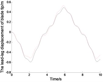
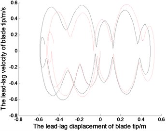
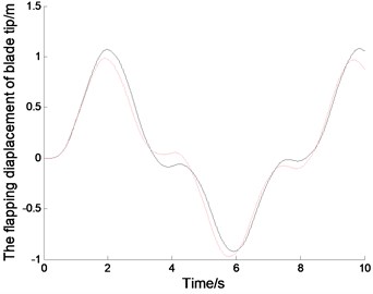
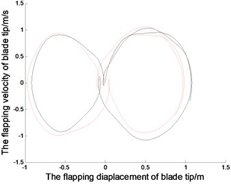
Fig. 2The displacements and phase tracks of blade tip (the red dotted line represents the linear system; the black solid line represents the nonlinear system)

The displacements and phase tracks of blade tip (the red dotted line represents the linear system; the black solid line represents the nonlinear system)

(a1)

(a2)

(b1)

(b2)

(c1)

(c2)

Fig. 2. represents the displacements and the phase tracks of the blade in the directions of lead-lag, flapping and twisting. The chosen parameters are $N =$ 30, $t_{h} =$ 0.001, $Ω =$ 0.8 rad/s. The initial displacements of blade tip are $U_{6} =$ –0.5432, $v_{6} =$ 2.0272, $φ_{6} =$ 0.2673. The initial displacements of other node must be selected by the linear vibration mode for the displacement continuity of continuous bar. The simulation of linear system can be achieved by Matlab/Simulink presented in [19-21]. In order to compare with linear system, the initial displacement of blade tip in nonlinear system should agree with that in linear system. But the initial displacement in other nodes will disagree with that in linear system with the nonlinear effect, which should be calculated according to nonlinear modes. Application of time discretion and Matlab vibration toolboxs, the wind turbine blade can be simulated in nonlinear autonomous system.

The Fig. 2. shows, in the linear system, the blade tip makes a simple harmonic vibration in the directions of lead-lag, flapping and twisting. The vibration period depends on the natural parameters of the blades. And initial displacement conditions determine the amplitudes of the blade vibration. In addition, the vibration characteristic of other positions in the blade is similar with that in blade tip, but the amplitudes are different. Because of nonlinear stiffness, the blade tip displacement in nonlinear system is sharper than that in linear system.With the nonlinear effect, the blade vibration is not strictly periodic motion, and the amplitudes of the vibration vary slightly. From the phase curves in Fig. 2. the vibration velocity of blade tip in nonlinear system is quite different from that in linear system. The displacements in positive and negative directions are different, but that in linear system are symmetrical.

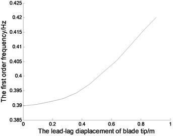
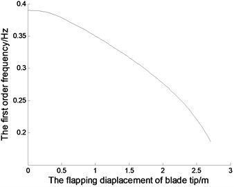
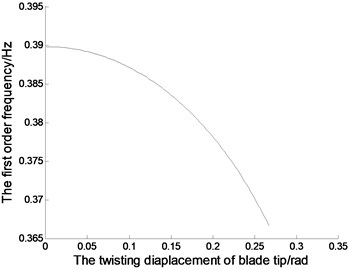
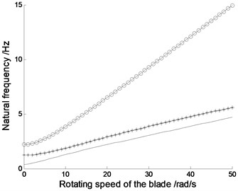
Fig. 3The nature frequencies of the blades (in Fig. 3(d), — – the first order nature frequency; * – the second order nature frequency; ○ – the third order nature frequency)

The nature frequencies of the blades (in Fig. 3(d), — – the first order nature frequency; * – the second order nature frequency; ○ – the third order nature frequency)

(a)

(b)

(c)

(d)

In Fig. 3(a), (b) and (c), $Ω =$ 0.8 rad/s. And the natural frequencies vary with the blade displacements in the directions of lead-lag, flapping and twisting. Fig. 3(a) shows, with increasing lead-lag diaplacements of blade tip, the natural frequencies increase accordingly. In Fig. 3(b) and Fig. 3(c), as increasing diaplacements of blade tip, the natural frequencies reduce in the directions of flapping and twistting. Fig. 3(d) shows, with increasing rotating speeds of the blade, all natural frequencies increase accordingly.And the change in third order natural frequency is quite obvious, that in first and second frequencies are not too obvious. The rotating speed of large horizontal axis wind turbine blades is relatively low, and the change range of which is limited in scope, so the rotating speed has little effect on the natural frequency of the blade.

Tables 1, 2 and 3 shows the first order nature frequencies with diffrenrent number of finite difference nodes and diffrenrent blade displacements in the directions of lead-lag, flapping and twisting, respectively. Table 3 shows the first order nature frequencies with diffrenrent number of finite difference nodes and diffrenrent rotating speeds. The higher the number of finite difference nodes is,the more exact the solution of the system is. When $N$ comes to a value,the increase of which can not enhance the precision of the computation obviously. With increasing finite difference nodes, the computing time will become long. So $N =$ 30 is a good choice for simulation of the systems.

Table 1The first order nature frequencies with different lead-lag diaplacements

Lead-lag displacement (m)	0	0.2	0.4	0.6	0.8
$N =$ 6	0.385435	0.391554	0.395111	0.403498	0.414723
$N =$ 10	0.385872	0.391776	0.395340	0.403746	0.414956
$N =$ 16	0.385932	0.391820	0.395434	0.403843	0.415024
$N =$ 30	0.385970	0.391851	0.395452	0.403872	0.415002
$N =$ 50	0.385971	0.391851	0.395451	0.403872	0.415001

Table 2The first order nature frequencies with different flapping diaplacements

Flapping displacement (m)	0	0.5	1.0	1.5	2.0
$N =$ 6	0.385435	0.370943	0.350499	0.320807	0.274704
$N =$ 10	0.385872	0.371167	0.350780	0.321067	0.274954
$N =$ 16	0.385932	0.371210	0.350821	0.321108	0.275012
$N =$ 30	0.385970	0.371231	0.350833	0.321124	0.275034
$N =$ 50	0.385971	0.371231	0.350833	0.321124	0.275035

Table 3The first order nature frequencies with different twisting diaplacements

Twisting displacement (m)	0	0.05	0.1	0.15	0.2
$N =$ 6	0.385435	0.388680	0.387423	0.384170	0.378041
$N =$ 10	0.385872	0.388812	0.387678	0.384314	0.378267
$N =$ 16	0.385932	0.388921	0.387756	0.384478	0.378314
$N =$ 30	0.385970	0.388940	0.387766	0.384474	0.378347
$N =$ 50	0.385971	0.388940	0.387766	0.384473	0.378347

Table 4The first order nature frequencies with different rotating speeds

Rotating speed (rad/s)	0.8	10	20	30	40
$N =$ 6	0.385435	1.55221	2.53160	3.29263	4.02112
$N =$ 10	0.385872	1.55445	2.53368	3.29599	4.02246
$N =$ 16	0.385932	1.55511	2.53434	3.29743	4.02303
$N =$ 30	0.385970	1.55526	2.53465	3.29762	4.02312
$N =$ 50	0.385971	1.55526	2.53465	3.29763	4.02312

5.3. Simulation on nonlinear non-autonomous system

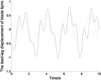
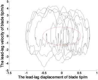
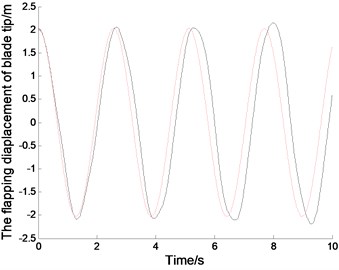
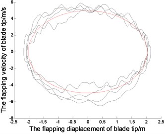
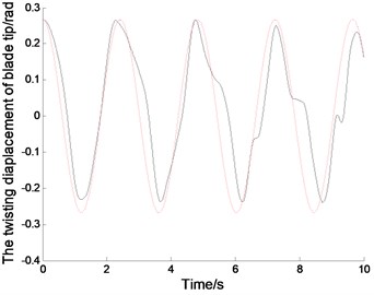
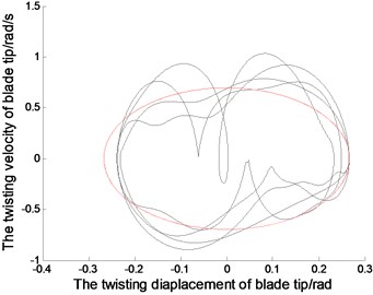
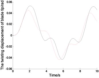
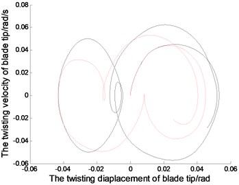
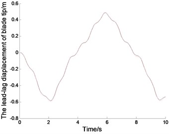
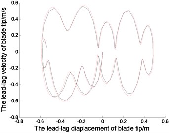
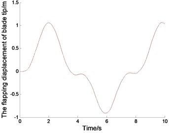
Considering gravity, the blade vibration equations by the finite difference discretization, can be described as a general nonlinear non-autonomous system. Application of time discretion and Matlab vibration toolboxs, the wind turbine blade can be simulated in nonlinear autonomous system. The chosen parameters are $N =$ 30, $t_{h} =$ 0.001, $Ω =$ 0.8 rad/s. The initial displacements of blade tip are zeros. Fig. 4 represents the displacements and the phase tracks of the blades in the directions of lead-lag, flapping and twisting.

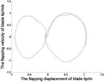
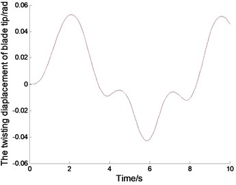
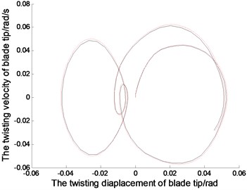
The displacements of the blades correspond to the sine excitation wih the gravity.When $Ω =$ 0.8 rad/s, the exciting period is 7.8555 s. Fig. 4(a1), (b1) and (c1) show the time displacement curves of the blade tip in non-autonomous system.The vibration of blade tip is basically sinusoidal, but there is a certain disturbance due to the coupling of vibration. The exciting period agrees with the vibration period in linear system, but slightly different from the vibration period in nonlinear system. Because of the nonlinear effects, nonlinear vibration amplitude is slightly different from the inear vibration amplitude. Fig. 4(a2), (b2) and (c2) show the phase tracks of the blade tip in non autonomous system, which not only reflect the relationships between the displacements and the velocities, but also can show the differences between the nonlinear vibration and the linear vibration.

Fig. 4The displacements and phase tracks of blade tip (the red dotted line represents the linear system; the black solid line represents the nonlinear system)

(a1)

(a2)

(b1)

(b2)

(c1)

(c2)

Fig. 5 shows the displacements and phase tracks of blade tip with diffrenrent $N$ and $t_{h}$ .The smaller the value of $t_{h}$ is, the more exact the solution of the system is. With decreasing time steps, the computing time will increase greatly. In Fig. 5(a2), the curve when $t_{h} =$ 0.001 is smoother than that when $t_{h} =$ 0.01. When $N$ or $t_{h}$ comes to a value, the change of which will have little effect on the calculation error. So $N =$ 30 and $t_{h} =$ 0.001, is chosen for simulation of the systems.

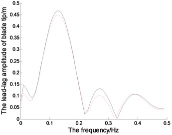
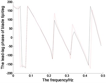
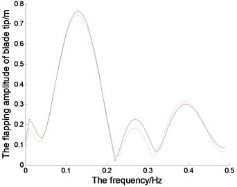
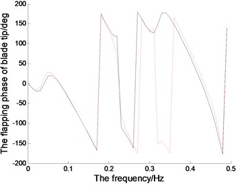
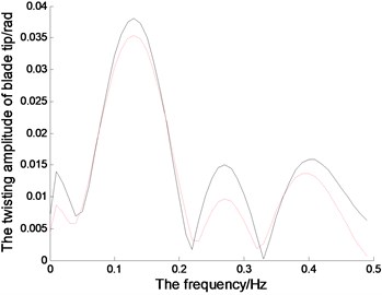
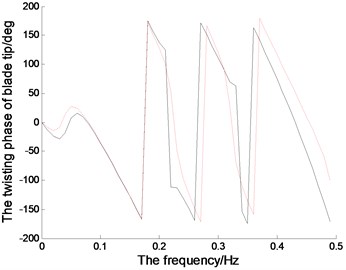
Fig. 6 represents the amplitude-frequency and phase-frequency characteristics of the blades in the directions of lead-lag, flapping and twisting,which is obtained through FFT transform of the vibration signal.When $Ω =$ 0.8 rad/s, excitation frequency is 0.1273 Hz, under which the blade will vibrate greatly. The first-order natural frequency of the blade is 0.39 Hz, in which the vibration amplitudes increase obviously.The nonlinear vibration amplitudes are bigger than those in linear system under those typical frequencies. And the blade phases in all directions change drastically in both nonlinear system and linear system under those typical frequencies.

Fig. 5The displacements and phase tracks of blade tip with diffrenrent N and th (the red dotted line represents N= 30 and th= 0.001; the black solid line represents N= 10 and th= 0.01)

The displacements and phase tracks of blade tip with diffrenrent N and th (the red dotted line represents N= 30 and th= 0.001; the black solid line represents N= 10 and th= 0.01)

(a1)

(a2)

(b1)

(b2)

(c1)

(c2)

Fig. 6The magnitude-frequency and phase-frequency characteristics of the blade tip (the red dotted line represents the linear system; the black solid line represents the nonlinear system)

The magnitude-frequency and phase-frequency characteristics of the blade tip (the red dotted line represents the linear system; the black solid line represents the nonlinear system)

(a1)

(a2)

(b1)

(b2)

(c1)

(c2)

6. Conclusions

According to Kallesøe’s model of turbine blades, two methods are developed to solve the nonlinear vibration of blades, namely, nonlinear non-autonomous system with gravity effect and nonlinear autonomous system without gravity effect. The equations are changed into the mass and stiffness matrices using a finite difference method on the boundary conditions of cantilever beams. This method has an exact solution, fast computation speed and wide application in the general nonlinear vibration theory.And the research work of the wind turbine blades is more comprehensive, and has an engineering significance.

By the time discretion methods and the Matlab vibration toolboxes, the displacements and the phase tracks of the blade tip are simulated in the directions of lead-lag, flapping and twisting. Then the amplitude-frequency and phase-frequency characteristic curves are plotted by the analysis of non-autonomous rotating turbine blades. Finally the simulation results are compared among the nonlinear systems and the linear systems. The nature frequencies and the nonlinear vibration characteristics are also discussed. This article can provide theoretical support for the design, operation, maintenance and flutter suppression on the large wind turbine blades.The nonlinear and linear simulation results not only show the difference between the linear system and the nonlinear system, but also can effectively verify the nonlinear vibration model and the validity of the algorithm. In addition, using a finite difference method to solve complex nonlinear problem of blade system is a beneficial attempt.

References

Chopra I., Dungundji J. Non-linear dynamic response of wind turbine blade. J. Sound Vib., Vol. 63, Issue 2, 1979, p. 265-286.

Search CrossRef
Hodges D. H., Dowell E. H. Nonlinear equation of motion for the elastic bending and torsion of twisted nonuniform rotor blades. NASA Tecnical Note, 1974, p. 19-25.

Search CrossRef
Hodges D. H., Robert A. Stability of elastic bending and torsion of uniform cantilever rotor blades in hover with variable structural couping. NASA Technical Note, 1976, p. 15-21.

Search CrossRef
Kallesøe B. S. Equations of motion for a rotor blade, including gravity, pitch action.Wind energy, Vol. 10, 2007, p. 211-216.

Search CrossRef
Shams S. H. Nonlinear aeroelastics response of slender wings based Wagner function. Thin Walled

Search CrossRef
Structures, Vol. 46, 2008, p. 1192-1203.

Search CrossRef
Tang D. M., Dowell E. H. S. Effects of geometric structural nonlinearity on flutter and lmit cycle oscillations of high-aspect-ratio wings. Journal of fluids and structures, Vol. 19, 2004, p. 291-306.

Search CrossRef
Huang J. L., Su R. K. L. Nonlinear vibration of a curved beam under uniform base harmonic excitation with quadratic and cubic nonlinearities. Journal of sound and vibraton, Vol. 330, 2011, p. 5151-5164.

Search CrossRef
Gunda J. B., Gupta R. K. Large amplitude vibration analysis of composite beams: simple closed-form solution. Composite, Vol. 93, 2011, p. 870-979.

Search CrossRef
Yang C. S., Xie Z. C. Perturbation method in the problem of large deflections of circular plates with nonuniform thickness. Applied Mathematics and Mechanics, Vol. 563, Issue 2, 1984, p. 1237-1242.

Search CrossRef
Marinca V., Herisanu N. A modified iteration perturbation method for some nonlinear oscillation problems. Acta Mechanica, Vol. 184, Issue 1-4, 2006, p. 231-242.

Search CrossRef
Jack K. H., Geneviève R. A Modified Poincaré Method for the Persistence of Periodic Orbits and Applications. Journal of Dynamics and Differential Equations, Vol. 22, Issue 1, 2010, p. 3-68.

Search CrossRef
Chen Y. Y., Chen S. H., Sze K. Y. A hyperbolic Lindstedt–Poincaré method for homo-clinic motion of a kind of strongly nonlinear autonomous oscillators. Acta Mechanica Sinica, Vol. 25, Issue 5, 2009, p. 721-729.

Search CrossRef
Xie L. H. The application of the asymptotic method to a clas of strongly nonlinear systems. Applied Mathematics and Mechanics, Vol. 14, Issue 9, 1993, p. 867-872.

Search CrossRef
Volkov V. T., Nefedov N. N. Development of the asymptotic method of differential inequalities for investigation of periodic contrast structures in reaction-diffusion equations. Computational Mathematics and Mathematical Physics, Vol. 46, Issue 4, 2006, p. 585-593.

Search CrossRef
Kalinin A. I. Asymptotic solution method for the control of the minimal force for a linear singularly perturbed system. Computational Mathematics and Mathematical Physics, Vol. 51, Issue 12, 2011, p. 1989-1999.

Search CrossRef
Moon B. Y., Kang B. S. Dynamic analysis of harmonically excited non-linear system using multiple scales method. Journal of Mechanical Science and Technology, Vol. 16, Issue 6, 2002, p. 819-828.

Search CrossRef
Niu B., JiangW. H. Multiple scales for two-parameter bifurcations in a neutral equation. Nonlinear Dynamics, Vol. 70, Issue 1, 2002, p. 43-54.

Search CrossRef
Derek B., Kevin J. Parametric study for large wind turbine blades. Sand 2002–2519 unlimited release printed, 2002, p. 12-18.

Search CrossRef
Kim T. Y. Nonlinear large amplitude structural and aeroelastic behhavior of cmposite totor blades at large static defection. Thin-Walled Structures, Vol. 46, 2008, p. 1192-1203.

Search CrossRef
Willam H. P., Saul A. T. Numerial recipes. 3rd ed. Cambridge: Cambridge Press publisher, 2007, p. 192-203.

Search CrossRef
Hansen M. H. Aeroelastic stability analysis of wind turbines using an eigenvalue approach.Wind Energy, Vol. 7, 2004, p. 133-143.

Search CrossRef

About this article

Received

16 May 2013

Accepted

05 November 2013

Published

31 December 2013

Keywords

vibration

horizontal axis

turbine blades

nonlinear

finite differential methods

Acknowledgements

This work was financially supported by the National Science Foundation (10972124) and Science and Technology Project of Department of Education of Shandong Province (J08LB04).

This is an open access article distributed under the Creative Commons Attribution License, which permits unrestricted use, distribution, and reproduction in any medium, provided the original work is properly cited.