Modal analysis of a cable-stayed bridge model using a modified Ibrahim Time domain algorithm

Modal analysis procedures are efficient techniques to identify modal properties of structures. The objective of this work is to conduct a vibration survey of a laboratory cable-stayed bridge model and to develop a systematic method for the extraction of the dynamic characteristics of the bridge model. The proposed method is based on the classical Ibrahim Time Domain (ITD) method and allows directly use the real time acceleration response measured from accelerometers due to ambient excitations. This is a clear advantage over classical ITD method. The feasibility and practicality are examined through a numerical study and an ambient modal testing of the bridge model. The modified method provides a very effective way to identify the dynamical properties of the structure. Modal analysis results shows that the bridge model is characterized by the presence of many closely spaced, coupled modes.

1. Outline

Structural health monitoring (SHM) of civil structures such as bridges, dams, and offshore platforms has been recently become a popular research issue [1]. A major engineering challenge associated with SHM is complete characterization of the dynamic response of the structure. A prerequisite of such applications is modal testing and analysis of the structure’s dynamic characteristics, including modal frequencies, mode shapes and modal damping ratios. Determination of the dynamic behavior of these structures under time-varying loads has become a practical engineering issue of worth attention.

Conducting dynamic testing is regarded as one of the most reliable experimental methods available for assessing actual dynamic properties of structures [2]. Such tests serve to complement and enhance the development of analytical techniques and models that are integral to analysis of the structure over its operational life. Ambient modal analysis techniques are particularly attractive to civil engineers, since the so-called output-only modal testing methods require no additional equipment to excite the structure being tested [3]. Techniques that utilize ambient excitations make use of pre-existing external forces resulting from wind loading, traffic loading, and ocean waves. Consequently, output-only methods are relatively nonintrusive and inexpensive as compared to the forced excitation methods.

During the past two decades, many researchers have conducted full-scale on-site dynamic tests on cable-stayed bridges. Typical examples of full-scale dynamic tests on bridges are provided in the References [4-7]. The peak-peaking technique [8] is one of the more widely used ambient modal analysis methods applied to the extraction of modal parameters of large civil engineering structures. Although the peak-peaking technique is straight forward, its accuracy of modal parameters estimation is known to rely heavily on the frequency resolution. A more advanced technique designed to overcome such difficulties is often cited in technical literature; this is Juang’s [9] eigensystem realization algorithm with data correlation (ERADC) method. The ERADC method is based on the realization algorithm, which is an identification process of a discrete state-space model from a pulse-response of a system. Although the ERADC method is systematic and relatively accurate, when a large number of time samples are collected at a large number of locations, the ERADC method requires heavy computations due to the singular value decomposition (SVD) process.

An outstanding progression in the frequency domain approach is the frequency domain decomposition (FDD) method by Brinker et al. [10]. The FDD method identifies the mode shapes and damped natural frequencies of a dynamic system by applying the SVD technique to the output spectral density matrix. This is done under an assumption of white noise excitation. The damping ratio and un-damped natural frequency are estimated from a mode-isolated, free-decay response obtained via an inverse Fourier transform of the output spectrums after applying a zero padding technique. Although the FDD method is much more advanced as compared to the peak picking method, the FDD method still requires a massive numerical computation attributable to the SVD process in the frequency domain.

One of the memorable efforts is the Ibrahim time domain (ITD) method developed by Ibrahim [11]. The ITD method uses Impulse Response Function (IRF) data to identify modal parameters. It constructs an eigenvalue problem from the IRF data and solves the problem to derive the natural frequencies, damping loss factors and modal constants. This modal parameter identification method is useful when the input data is unknown, in particular in structural dynamical testing under ambient loads, and thus chosen for dynamical analysis in this study. However, this method, when originally proposed, constructs the eigenvalue problem using displacement, velocity IRF data. As a result, numerical integration is needed to obtain displacement and velocity time histories from acceleration measurement at each response point. In addition, one of difficulties of the ITD method is the occurrence of fictitious modes that are caused by either noise or other irregularities in the measured data [12].

In this paper, a modified ITD method is developed in a way similar to that proposed in Ref. [11], but based on the sampling measured data in acceleration form to extract modal parameters using output-only responses. In addition to the modified ITD method, a mode shape coherence and confidence factor (MSCCF) will also be given to distinguish genuine modes from fictitious modes. The following three steps are performed to achieve this objective. First, the theoretical background of the modified ITD technique is presented. Second, use of the technique is demonstrated through a numerical simulation based a finite element (FE) analysis. Third, the feasibility and practicality of the proposed technique are examined using data taken on a cable-stayed bridge model. The paper concludes with a discussion on the modal analysis results obtained using the modified ITD method, including observation of the mode coupling interaction between bridge tower and deck vibrations.

2. Theoretical background

In this paper, the ITD approach is improved by directly using the real time acceleration signals. The deficiency of the amount of data needed is remedied by sampling the displacement data with a selected time delay. The free response of a structure means either the free decays measured from random execution of the structure or the impulse response obtained from the inverse of a frequency response function (FRF). In the following, we discuss this modified time domain method which is efficient for modal analysis.

2.1. Classical ITD method

The free displacement response of a N-DOF viscous damping system can be represented with the following formula according to the principle of mode superposition:

1

[X (t_{i})] = \sum_{i = 1}^{n} (ϕ_{i} e^{λ_{i} t_{i}} + ϕ_{i}^{*} e^{λ_{i}^{*} t_{i}}) .

Eq. (1) is a conjugate relationship and can be simplified into a new form:

2

[X (t_{i})] = \sum_{i = 1}^{2 n} Φ_{i} e^{λ_{i} t_{i}} .

Eq. (2) is based on the displacement $X (t_{i})$ . The acceleration $X (t_{i})$ can be derived from twice derivative of displacement data in the following form:

3

[\ddot{X} (t_{i})] = \frac{d^{2} [X (t_{i})]}{d t_{i}^{2}} = \sum_{i = 1}^{2 n} Φ_{i} λ_{i}^{2} e^{λ_{i} t_{i}} .

When the measuring point is $N$ , the sampled discrete points is $M$ , Eq. (3) can be expressed as:

4

[\begin{matrix} {\ddot{X}}_{1,1} & {\ddot{X}}_{1,2} & \dots & {\ddot{X}}_{1, M} \\ {\ddot{X}}_{2,1} & {\ddot{X}}_{2,2} & \dots & {\ddot{X}}_{2, M} \\ ⋮ & ⋮ & ⋱ & ⋮ \\ {\ddot{X}}_{N, 1} & {\ddot{X}}_{N, 2} & \dots & {\ddot{X}}_{N, M} \end{matrix}] = [\begin{matrix} ϕ_{1,1} & ϕ_{1,1}^{*} & \dots & ϕ_{1, N}^{*} \\ ϕ_{2,1} & ϕ_{2,1}^{*} & \dots & ϕ_{2, N}^{*} \\ ⋮ & ⋮ & ⋱ & ⋮ \\ ϕ_{N, 1} & ϕ_{N, 1}^{*} & \dots & ϕ_{N, N}^{*} \end{matrix}]

* [\begin{matrix} λ_{1}^{2} & 0 & \dots & 0 \\ 0 & {(λ_{1}^{*})}^{2} & \dots & 0 \\ ⋮ & ⋮ & ⋱ & ⋮ \\ 0 & 0 & \dots & {(λ_{N}^{*})}^{2} \end{matrix}] [\begin{matrix} e^{λ_{1} t_{1}} & e^{λ_{1}^{*} t_{2}} & \dots & e^{λ_{1} t_{M}} \\ e^{λ_{1}^{*} t_{1}} & e^{λ_{1}^{*} t_{2}} & \dots & e^{λ_{1}^{*} t_{M}} \\ ⋮ & ⋮ & ⋱ & ⋮ \\ e^{λ_{N}^{*} t_{1}} & e^{λ_{N}^{*} t_{2}} & \dots & e^{λ_{N}^{*} t_{M}} \end{matrix}] .

It can be simplified as following formula:

5

{[\ddot{X}]}_{N, M} = {\hat{Φ}}_{N, 2 N} Γ_{2 N, M} = Φ_{N, 2 N} \nabla_{2 N, 2 N} Γ_{2 N, M} .

This equation establishes direct links between the complex natural frequencies, mode shapes and the time response of the system. It alone, however, is insufficient to solve for modal data. The approach is to sample the same response data but with a duration shift $Δ t$ .

For all the response points, through using a delayed sampling for $Δ t_{1}$ , which is the integer multiple of $Δ t$ , a vector form of Eq. (5) can be written as:

6

{[\ddot{Y}]}_{N, M} = [\ddot{X} (t_{i} + {Δ t}_{1})] = \sum_{i = 1}^{2 N} {\hat{Φ}}_{i} e^{λ_{i} (t_{i} + {Δ t}_{1})},

where:

7

{[\ddot{Y}]}_{N, M} = {\hat{Φ}}_{N, 2 N} [\begin{matrix} e^{λ_{1} {Δ t}_{1}} & 0 & \dots & 0 \\ 0 & e^{λ_{1}^{*} {Δ t}_{1}} & \dots & 0 \\ ⋮ & ⋮ & ⋱ & ⋮ \\ 0 & 0 & \dots & e^{λ_{N}^{*} {Δ t}_{1}} \end{matrix}] Γ_{2 N, M} .

Using a delayed sampling matrix ${[\ddot{Y}]}_{N, M}$ and normal sampling matrix ${[\ddot{X}]}_{N, M}$ to construct augmented matrix:

8

{[Q_{\ddot{X} \ddot{Y}}]}_{2 N, M} = [\begin{matrix} \ddot{X} \\ \ddot{Y} \end{matrix}] = [\begin{matrix} {\hat{Φ}}_{N, 2 N} Γ_{2 N, M} \\ {\hat{Φ}}_{N, 2 N} Δ_{2 N, 2 N} Γ_{2 N, M} \end{matrix}] = [ϒ_{2 N, 2 N}] [Γ_{2 N, M}] .

Likewise, we can increase the time shift to ${Δ t}_{2}$ , which is the integer multiple of ${Δ t}_{}$ and may be equal or not be equal to ${Δ t}_{1}$ , and sample the response data again. For all the response points, a vector can be written as:

9

{[{\tilde{Q}}_{\ddot{X} \ddot{Y}}]}_{2 N, M} = [\begin{matrix} \ddot{X} (t_{i} + {Δ t}_{2}) \\ \ddot{Y} (t_{i} + {Δ t}_{2}) \end{matrix}], {[{\tilde{Q}}_{\ddot{X} \ddot{Y}}]}_{2 N, M} = [\begin{matrix} {\hat{Φ}}_{N, 2 N} Ω_{2 N, 2 N} Γ_{2 N, M} \\ {\hat{Φ}}_{N, 2 N} Δ_{2 N, 2 N} Ω_{2 N, 2 N} Γ_{2 N, M} \end{matrix}],

where:

10

{[{\tilde{Q}}_{\ddot{X} \ddot{Y}}]}_{2 N, M} = [{\tilde{ϒ}}_{2 N, 2 N}] [Γ_{2 N, M}], [{\tilde{ϒ}}_{2 N, 2 N}] = [ϒ_{2 N, 2 N}] [Ω_{2 N, 2 N}],

where $Ω_{2 N, 2 N}$ is:

11

[Ω_{2 N, 2 N}] = [\begin{matrix} e^{λ_{1} {Δ t}_{2}} & 0 & \dots & 0 \\ 0 & e^{λ_{1}^{*} {Δ t}_{2}} & \dots & 0 \\ ⋮ & ⋮ & ⋱ & ⋮ \\ 0 & 0 & \dots & e^{λ_{N}^{*} {Δ t}_{2}} \end{matrix}] .

According to the relationship between augmented matrix $Q_{\ddot{X} \ddot{Y}}$ with ${\tilde{Q}}_{\ddot{X} \ddot{Y}}$ , we have:

12

{\tilde{Q}}_{\ddot{X} \ddot{Y}} Q_{\ddot{X} \ddot{Y}}^{- 1} ϒ_{2 N, 2 N} = ϒ_{2 N, 2 N} Ω_{2 N, 2 N} .

Defining that:

13

A = {\tilde{Q}}_{\ddot{X} \ddot{Y}} Q_{\ddot{X} \ddot{Y}}^{- 1} .

In actual application, the sampled discrete points $M$ is larger than 2 times of the measuring points $N$ ( $M > 2 N$ ), so the structural system matrix $A$ can be achieved by the least squares method to reduce error. Eq. (12) can be simplified as:

14

A ϒ_{2 N, 2 N} = ϒ_{2 N, 2 N} Ω_{2 N, 2 N} .

Because $Ω_{2 N, 2 N}$ is a diagonal matrix, the Eq. (14) is equivalent to:

15

A ϒ_{2 N, 2 N} = Ω_{2 N, 2 N} ϒ_{2 N, 2 N} .

This equation constitutes a complex eigenvalue problem ( $Ω_{2 N, 2 N}$ contains structural modal frequency and modal damping ratios; $ϒ_{2 N, 2 N}$ contains structural mode shapes). These eigenvalues can be converted to the natural frequencies and damping ratio.

2.2. Modification of classical ITD method

The classical ITD algorithm [11] uses the displacement response of several outputs in order to find modal parameters. The modified ITD method presented next uses an approach similar to the classical ITD, but the identification is based on the acceleration response in an explicitly way, and more feasible for ambient vibration techniques in practice.

The $i$ th diagonal element in Eq. (11) is the eigenvalue in the form:

16

Ω_{i} = e^{λ_{i} {Δ t}_{2}},

and:

17

λ_{i} = \frac{l n (Ω_{i})}{{Δ t}_{2}} .

From these solutions, we can derive the undamped modal frequency $ω_{d i}$ and modal damping ratio $ε_{d i}$ :

18

ω_{d i} = \frac{| λ_{i} |}{2 π},

19

ε_{d i} = \sqrt{\frac{1}{1 + \frac{I m (λ_{i})}{R e (λ_{i})}}} .

And the structural mode shapes $ϒ_{i}$ are:

20

ϒ_{i} = \frac{1}{λ_{i}^{2}} [\begin{matrix} {\hat{ϕ}}_{i} \\ φ_{i} \end{matrix}] .

Complex mode shapes vector is the first $N$ elements array based on the acceleration signal ( $i =$ 1, 2,…, 2 $N$ ). Using the augmented matrix [ $Q$ ] to replace [ $X$ ] in the analysis described from Eqs. (3)-(9) will lead to the identification of many numerical vibration modes as well as genuine modes.

To distinguish the latter from the former, a mode shape coherence and confidence factor (MSCCF) can be defined. For a selected measurement point, the MSCCF defined as:

21

M S C C F = \frac{{(ϒ_{k}^{u})}^{T} {(ϒ_{k}^{l})}^{*} e^{λ_{k} {Δ t}_{1}}}{{(ϒ_{k}^{l})}^{T} {(ϒ_{k}^{l})}^{*}},

where $ϒ_{k}^{u}$ is the upper half part of the $k$ order mode, and $ϒ_{k}^{l}$ is the lower half part of the $k$ order mode. If the mode is a genuine one, $M S C C F$ will be close to unity. Otherwise, it is likely the mode is a numerical one. In practical engineering applications, the measured data always contains noise. In this case, if the value of MSCCF is more than 0.95, it can be regarded as a genuine one.

3. Numerical example

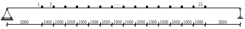
The technique discussed above was programmed using MATLAB and applied to the analysis of a simply supported beam using the FE software package ANSYS. Consider the simple supported beam shown in Fig. 1. The length of the beam is 20 m, and 15 accelerometers are placed on the beam with an equal spacing of 1 m. The second moment of cross-sectional area, Young’s modulus, and density of the beam are 0.28 m⁴, 20 GPa, and 8.5×10³ kg/m³, respectively. The finite element (FE) model consists of 100 linear elements (101 nodes), each with a uniform length of 0.2 m. From the FE analysis, the un-damped natural frequencies for the first, second, and third bending modes are 2.58 Hz, 10.07 Hz, and 21.76 Hz, respectively.

Fig. 1Simulated sensor location of the beam

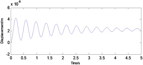
Given a unit pulse load at the third sensor, the acceleration time responses at all of the sensors are simulated. The damping ratio used here is 0.03 (a typical value for lightly damped structures) for all modes. With a sampling frequency of $f_{s} =$ 300 Hz, transverse degrees of freedom are collected at the 15 sensor locations. The typical acceleration time history and its corresponding displacement time history at the fourth node are shown in Figs. 2 and 3, respectively. Using the acceleration time history records, the modal frequencies of the beam are determined by executing the modified ITD method. The modal parameters have also been computed by the classical ITD method using displacement time history records. In addition, in order to investigate the sensitivity of the identification to the accuracy of the structural natural frequency, 10 % and 20 % white noises are introduced in this study.

Fig. 2Acceleration at the fourth node of the beam

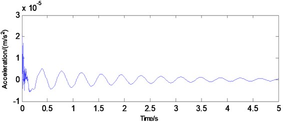
Fig. 3Displacement at the fourth node of the beam

The identified modal frequencies from both methods is listed in Table 1 and can be seen to be very close to the frequency of the FE results. In the case of without noise, results of the modified method are slightly better than identification results obtained with classical approach. However, in other cases, it is observed that classical ITD algorithm applied to the displacement records do not work well in the presence of noises. The new method applied to the acceleration records is able to provide reliable modal parameters in those cases. Hence, the proposed modified ITD method shows better robustness with respect to real application for structure operational setting.

Table 1The identified first three modal frequencies

Order		FEA (Hz)	Without noise		With 5 % noise		With 10 % noise
Order		FEA (Hz)	Frequency (Hz)	Error %	Frequency (Hz)	Error %	Frequency (Hz)	Error %
1	Acceleration	2.58	2.58	0.00	2.62	1.64	2.65	2.71
1	Displacement	2.58	2.59	0.39	2.64	2.49	2.52	6.15
2	Acceleration	10.07	9.69	3.78	10.96	8.79	10.01	8.56
2	Displacement	10.07	9.53	5.37	11.02	9.43	9.07	9.93
3	Acceleration	21.76	22.02	1.21	21.39	1.70	21.09	3.08
3	Displacement	21.76	22.92	5.33	23.34	7.26	23.99	10.25

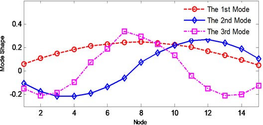
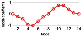
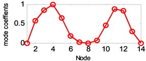
The next step involves performing a modified ITD analysis on damping ratios and mode shapes of the structure. Note that the size of matrix for the modified ITD analysis is only 15×15 for each mode. For each mode, the 15×1 un-damped mode shapes vector is extracted by taking the first column vector in Eq. (20). The first three bending mode shapes to be identified are shown in Fig. 4. Using Eq. (19), the corresponding damping ratios determined with the modified ITD method are 2.08 %, 0.25 %, and 0.04 %, respectively. It can be seen in this numerical study that the modified ITD method rely on the acceleration responses is straightforward and more accurate compared to the classical method.

Fig. 4The estimated first three bending modes of the beam using the modified ITD

4. Experimental validation

4.1. Description of test structure

As shown in Fig. 5, the bridge model represents a reduced-scale model of Shandong Binzhou Yellow River cable-stayed bridge (see Fig. 6). This single-tower double-cable-planes bridge model is mainly made of aluminum. Effective stiffness criterion is utilized in the reduced-scale dynamic-elastic bridge model design. Additional masses are added so the bridge model would give similar dynamic characteristics within the range of the prototype bridge. The bridge model is eventually built in a ratio of 1/40 to the prototype bridge considering lab conditions and economic. Table 2 lists the specific parameters of the bridge model. Several experiments have been previously conducted with various configurations of this structure [13]. Their analysis results based on the similarity theory have showed that the reduced-scale bridge model with added masses has a good degree of similarity with the prototype bridge.

Fig. 5Binzhou Yellow River bridge

Fig. 6The reduced-scale laboratory bridge model

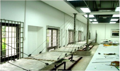
Table 2Experimental cable-stayed bridge model mechanical characteristics

Element	Cross section	Material	Density (kg/m³)	Modulus (GP)	Poisson ratio	Dimension (m)
Middle tower	Box	Aluminum alloy	2700	68.6	0.34	3.1×0.1375×0.095
Side tower	Box	Aluminum alloy	2700	68.6	0.34	1.9×0.12×0.075
Deck	Separate box	Aluminum alloy	2700	68.6	0.34	15.2×0.82×0.07
Cable	Circle ○	High-strength steel wire	7850	200	0.30	Varies

4.2. Establish FEM model

Motivation of the use of a FE model is its capability of accurate assessment of bridge model modal properties. Such properties are integral to providing a reference for investigation of above proposed new method and to assess the condition of the structure over its operational life.

Fig. 7Cable-stayed bridge analysis model of three-dimensional finite element

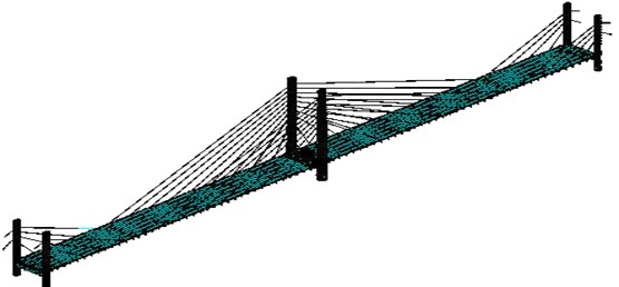
Table 3Vibration modes of bridge model results from FE analysis

Order	Modes category	Frequency (Hz)	Order	Modes category	Frequency (Hz)
1	Deck first anti-symmetric vertical bending	4.56	6	Tower first symmetric sidesway	12.50
2	Deck first anti-symmetric torsion	9.10	7	Tower first anti-symmetric sidesway	12.57
3	Deck first symmetric vertical bending	9.24	8	Deck first torsion	13.58
4	Deck second order anti-symmetric vertical bending	11.09	9	Deck third order anti-symmetric vertical bending	14.59
5	Deck second order symmetric vertical bending	11.99	10	Deck third order symmetric vertical bending	15.55

A three-dimensional FE model is established in ANSYS, shown in Fig. 7. The geometry and member details of the model are based on the design information of the bridge model. The initial force in the cables and the gravity of the bridge has little effect on the dynamic characteristics of the structure [14]. Therefore, the initial force in the cable and gravity of the bridge can be ignored when modal analysis carried out. By constraining the corresponding nodes’ degree, the boundary conditions of the model can be defined. The main structural members are composed of stay cables, floor beams, and towers, all of which are discreterized by different finite element types. Modeling of the stay cables is possible in ANSYS by employing the 3-D tension-only truss elements (LINK10), and utilizing its stress-stiffening capability. Each stay cable is modeled by one element, which results in 60 tension-only truss elements in the model. Two steel main girders are modeled as the 3-D elastic beam elements (BEAM188) for simplicity, since they are the structural members possibly subjected to tension, compression, bending and torsion. Towers consist of both equivalent and variable sections so they are discreterized by BEAM188 elements. There are in total 1498 elements of this type. The deck modeled by the shell elements (SHELL63) with a total number of 1512. All piers and platforms are modeled by the solid elements (SOLID45), of which there are 852. The diaphragms are modeled by 80 beam elements (BEAM44). In addition, 210 concentrated mass elements (MASS21) are used to include the mass of equilibrium blocks, parapet and anchors that are nonstructural members. The complete model consists of 1371 nodes and 1500 elements resulting in 8202 active degrees of freedom (DOFs). After performing a modal analysis in ANSYS, the first ten mode shapes and natural frequencies of the bridge model are listed in Table 3. The FE analysis generates a total of ten vibration modes within the frequency range of 0.4-2.5 Hz, indicating closely spaced natural frequencies. They are classified as: five vertical predominant modes, six lateral modes, and two tower modes.

4.3. Description of modal test

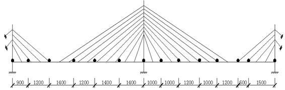
A set of nearly identical ambient vibration tests are scheduled to record acceleration time responses of the test structure. Two electronic-dynamic shakers were applied underneath the structure to provide white-noise loads by shaking the bridge deck up-down, as would be done in a normal operational setting. 14 piezoelectric accelerometers are distributed along the center line of the bridge model in a pattern established to derive the operational mode shapes. The sensor layout and excitation points are shown in Fig. 8. All records are sampled using the standard sampling frequency of 1000 Hz and baseline-corrected before processing. The duration of each record is 20 sec. A user-friendly LabVIEW graphical user interface is developed to control the vibration generator and collect the structural dynamical responses.

Fig. 8Sensor layout physical location

4.4. Modal analysis using proposed method

Table 4Modal parameters of bridge model identified using modified ITD

Order	Frequency (Hz)	Damping ratio	MSCCF
1	3.97 (deck)	7.69 %	0.987
2	8.63 (deck)	0.51 %	0.999
3	10.52 (deck)	0.66 %	0.999
4	11.62 (deck)	0.55 %	0.999
5	15.04 (deck)	0.48 %	0.998
6	16.12 (deck)	0.46 %	0.999
7	9.89 (tower)	0.41 %	0.981
8	10.62 (tower)	0.52 %	0.946

Using only output acceleration time histories processed with the modified ITD technique, natural frequencies and associated damping ratios of bridge deck and tower are extracted and listed in Table 4. For the frequency zone, the estimated natural frequencies for the first six vertical bending modes, using the modified ITD method are 3.97, 8.63, 10.52, 11.62, 15.04, and 16.12 Hz, respectively. The corresponding modal damping ratios are 7.69 %, 0.51 %, 0.66 %, 0.55 %, 0.48 %, and 0.46 %, respectively. In order to distinguish the genuine mode from the numerical vibration modes due to the augmented measurement data in the proposed algorithm, the MSCCF, a modal confidence factor, was defined and computed before the identification of mode shapes from the test data. For the six extracted mode shapes, the MSCCF values are 0.987, 0.999, 0.999, 0.999, 0.999, and 0.999, respectively. Note that the MSCCF values identified are nearly equal to unity in all cases. Therefore, the new method proposed here is able to provide reliable modal parameters in those cases. While there are no repeated modes, there are very close natural frequencies of the bridge model.

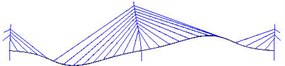
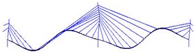
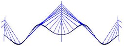
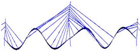
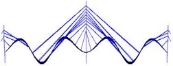
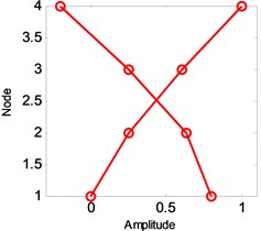
Fig. 9Mode shapes from FEM analysis

a) 1st vertical mode

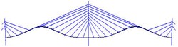
b) 2nd vertical mode

c) 3rd vertical mode

d) 4th vertical mode

e) 5th vertical mode

f) 6th vertical mode

g) Tower first symmetric sidesway

h) Tower first anti-symmetric sidesway

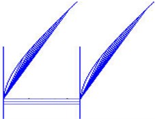
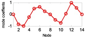
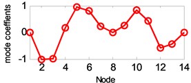
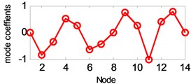
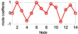
Fig. 10Mode shapes from modified ITD

a) 1st vertical mode

b) 2nd vertical mode

c) 3rd vertical mode

d) 4th vertical mode

e) 5th vertical mode

f) 6th vertical mode

g) Tower first symmetric sidesway

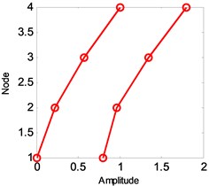
h) Tower first anti-symmetric sidesway

While the identification method can simultaneously generate the global modes, the local modes of structural members can also be identified by employing the sensors associated only with those of the members. In this section, the deck modes and tower modes are examined. Considering the rigid shape of the deck, especially the fixed connection between the tower and deck, and the longitudinal restraints, domination of vertical vibration is expected. For this purpose, sensors measure accelerations of deck in vertical direction and tower in lateral direction are utilized as outputs.

The estimated six vertical bending mode shapes of deck and two sideway mode shapes of tower are present in Fig. 10. Their mode shapes fit their FEM counterparts mode shapes very well. The results are completely symmetrical or anti-symmetric, which present the structural characteristic of the cable-stayed bridge. The fundamental mode of the bridge is the first vertical bending with a natural frequency of 3.97 Hz. This mode exhibits a zero node symmetrical pattern of girder. The results of modal analysis of the tower indicate that the first and second modes are dominated by lateral motion, with the difference in the phase. The first mode exhibits an in-phase motion, while the second one shows the out-of-phase motion. Both tower modes at the frequency range of 9.89-10.62 Hz are associated with the deck motion. The interactions between the deck motion and tower exist in such a way that the tower modes are resulted from their girder’s predominant counterpart modes. Damping ratios of tower modes are found lower than the deck modes. The damping ratios of the first two lateral modes identified at tower are 0.41 % and 0.52 %.

5. Conclusions

In this paper, a modified ITD algorithm has been introduced in modal analysis of a laboratory cable-stayed bridge, based on the classical ITD algorithm. The proposed method provides a very effective way to identify the modal parameters of the structure through the spatially distributed sensors. A FEM model of cable-stayed bridge is established, and modal analysis is carried out for the cable-stayed bridge model. The following conclusions are drawn from modal analysis made on the bridge model:

1) The modified ITD method has several advantages over its classical counterpart. It does not need numerical integration to obtain displacement and velocity time histories from acceleration measurement at each response point. Results of the modified method are slightly better than identification results obtained with a standard approach. It is possible to use this technique for modal analysis based real time structural health monitoring.

2) Ideally, the proposed method requires data measured from all measurement points on a structure simultaneously. This avoids unnecessary phase difference among responses and ensures that all responses come from the same initial forcing conditions. In reality, it may not be practical to measure many channels of responses at the same time due to hardware limitations.

3) The results of modal analysis have provided conclusive evidence of the complex dynamic behavior of the bridge. The dynamic response of the cable-stayed bridge is characterized by the presence of many closely spaced, coupled modes. For most modes, the analytical and the experimental modal frequencies and mode shapes compare quite well. Based on the analysis of ambient vibration data, it is evident that the vertical vibration of the bridge deck is tightly coupled with the tower vibrations within the frequency range of 9-11 Hz.

4) As for the damping ratio estimation, the first vibration mode of the deck had a damping ratio of 7.69 % on average (depends upon the different sensor locations); the damping values for higher modes are less than 1.0 %. More detailed study on the estimation of accurate damping ratios is needed in future research.

References

Farrar C. R. Historical overview of structural health monitoring. Journal of Lecture Notes on Structural Health Monitoring Using Statistical Pattern Recognition, Los Alamos Dynamics, Los Alamos, NM, USA, 2001.

Search CrossRef
Liu C. Y., Olund J., Cardini A., et al. Structural health monitoring of bridges in the State of Connecticut. Journal of Earthquake Engineering and Engineering Vibration, Vol. 7, Issue 4, 2008, p. 427-37.

Search CrossRef
Liu C. Y., DeWolf J. Effect of temperature on modal variability of a curved concrete bridge under ambient loads. Journal of Structural Engineering, Vol. 133, Issue 12, 2007, p. 1742-1751.

Search CrossRef
Ko J. M., Sun Z. G., Ni Y. Q. Multi-stage identification scheme for detecting damage in cable-stayed Kap Shui Mun Bridge. Engineering Structures, Vol. 24, Issue 7, 2002, p. 857-68.

Search CrossRef
Ozkan E., Main J., Jones N. P. Long-term measurements on a cable-stayed bridge. Conference on Structural Dynamics, 2001, p. 518-523.

Search CrossRef
He X., Moaveni B., Conte J. P., et al. System identification of New Carquinez Bridge using ambient vibration data. International Conference on Experimental Vibration Analysis for Civil Engineering Structures, 2005, p. 26-28.

Search CrossRef
Wenzel H., Pichler D. Ambient Vibration Monitoring. John Wiley & Sons, 2005.

Search CrossRef
Bendat J. S., Piersol A. G. Engineering Applications of Correlation and Spectral Analysis. Wiley, New York, 1980, p. 181-186.

Search CrossRef
Juang J. N. Applied system identification. Prentice-Hall, Englewood Cliffs, NJ, 1994, p. 133-147.

Search CrossRef
Brinker R., Zhang L., Andersen P. Modal identification from ambient responses using frequency domain decomposition. Proceedings of 18th International Modal Analysis Conference, San Antonio, 2000, p. 625-30.

Search CrossRef
Ibrahim S. R., Mikulcik E. C. A method for the direct identification of vibration parameters from the free response. Shock and Vibration Bulletin, Vol. 47, Issue 4, 1977, p. 183-198.

Search CrossRef
Ewins D. J. Modal Testing: Theory, Practice and Application. Research Studies Press, Hertfordshire, England, 2000.

Search CrossRef
Zhou L. R., Yang O., Ou J. P. Design and analysis of laboratory health monitoring model of a long-span cable-stayed bridge. Proceedings of the 20th National Compilation of Vibration and Noise of High Technology and Application Conference, 2007, p. 57-66.

Search CrossRef
Liu S. L.,Wang S. H. The Designing of Cable-stayed Bridge. Beijing. People’s Communications Press, 2006.

Search CrossRef

About this article

Received

19 March 2014

Accepted

26 May 2014

Published

30 September 2014

Keywords

modal analysis

Ibrahim Time Domain

modal testing

dynamical property

Acknowledgements

Financial supports from the National Science Foundation of China (No. 51108129), Shenzhen Overseas Talents Project (Grant No. KQCX20120802140634893), and Guangdong Science and Technology Major Project (No. 2012A080104014) to initiate this research project are greatly acknowledged.

This is an open access article distributed under the Creative Commons Attribution License, which permits unrestricted use, distribution, and reproduction in any medium, provided the original work is properly cited.