Abstract
The multi-objective optimization configurations of thickness, the locations of constrained layer damping (CLD) patches for plate are investigated and the vibration characteristics of the CLD/plate are analyzed based on the Pareto optimal solutions. The finite element method, in conjunction with the Golla-Hughes-McTavish (GHM) method, is employed to model the plate with CLD treatments to predict its vibration characteristics. A multi-objective optimization model for CLD/plate is formulated based on the dynamical equation. The design objectives are to maximize the mode loss factors, while the design variables include the thicknesses of viscoelastic material (VEM) and constrained layer material (CLM), the locations of CLD treatments on the plate. Aiming to the special real-integer hybrid variables optimization problems, the non-dominated sorting genetic algorithm II (NSGA-II) is employed and improved. Two different optimization strategies are proposed. As the results of the numerical example, the various feasible Pareto optimal solutions are successfully obtained, and effects of the design variables on the vibration characteristics are discussed. The influences of algorithm parameters on the optimization procedure are also investigated. The results show the validity of improved NSGA-II and the optimization strategies. The potential multiple selections of CLD treatments for different vibration control objectives and constrained conditions are also demonstrated.
1. Introduction
Vibration control of flexible structure is a common subject of engineering community. Active Constrained Layer Damping (ACLD) treatment has been used widely for damping the vibration of beams [1, 2], plates [3] and shells [4]. Such a system generally comprises a layer of viscoelastic material (VEM) sandwiched between a host structure and an active cover sheet, such as a piezoelectric layer.
The overall performance of the ACLD system is governed by performance of the passive (open-loop) and the active controls (closed-loop). Thus, the optimization for the ACLD system consists of two parts, specifically, optimum design of the open-loop ACLD system, i.e. CLD system, and the closed-loop system. Optimization for CLD system is essential to enhance the performance of ACLD system. Furthermore, with optimally designed CLD treatments, the performance is guaranteed to be robust even if the active component of the ACLD ceases to operate or fail [5]. In the case of optimum design of CLD system, extensive efforts have been exerted to optimally design CLD treatment subject to space or weight limitations [6-8]. Parametric studies regarding variations in the natural frequencies and the mode damping ratios or loss factors have been implemented. Kung and Singh [9] developed an energy-based approach of multiple constrained layer damping patches. They only investigated the effect of constrained layer damping patches on suppressing vibration of several modes separately. Baz [5] optimized the placement of ACLD patches using the mode strain energy (MSE) method. In this study, the total weight of the damping treatments was taken as the objective function while satisfying constraints imposed on the mode damping ratios. Zheng and Cai [10] employed four different nonlinear optimization methods/algorithms (sub-problem approximation method, the first-order method, sequential quadratic programming (SQP) and genetic algorithm (GA)) to find the optimal locations and lengths of the CLD patches, to minimize displacement amplitude at the middle beam. Al-Ajmi and Bourisli [11] optimized CLD segments’ length using the genetic algorithm (GA). The optimization procedure was only able to identify a distribution of segments for a single mode. Zheng Ling [12] proposed an optimality criterion to find the optimal placement of CLD patches on the cylindrical shell. Li Yinong and Xie Ronglu [13] considered the CLD structure optimization as a topology optimization problem, and the evolutionary structural optimization (ESO) method was employed to find the optimal configuration of the CLD patches. Both papers took the mode loss factors as objective functions. Lepoittevin Grégoire and Kress, Gerald [14] proposed a new arrangement method for enhancement of damping capabilities of segmented CLD treatments, and a mathematical programming method was developed in order to get the optimal arrangement that optimized the mode loss factor. As mentioned above, locations of the CLD patches, thicknesses of the CLD and VEM were optimized, but there is a limitation that all the parameters were rarely taken as the optimal design variables at the same time. Additionally, many of them just took a single objective function to find the optimal configurations of CLD treatments.
In the present work, the objective is to develop a multi-objective optimization procedure for CLD structure with the ability to optimize locations of the CLD patches and thicknesses of the VEM and CLM simultaneously. Furthermore, effect of the parameters on vibration suppression performance can be analyzed based on Pareto optimal solutions set.
This paper is organized in six sections. In section 1, the brief introduction is given. In section 2, the finite element model of the CLD/plate is developed. In section 3, a multi-objective optimization model is established and two optimization strategies are proposed. Locations of CLD patches expressed by positive integers, and thicknesses of VEM and CLM which are presented by positive consequent-real numbers, constitute the hybrid variables. The mode loss factors are served as objective functions, the added-mass and frequency shift are taken as constraint conditions. To obtain the optimal configuration of CLD treatments, the improved NSGA-II (INSGA-II) is proposed and explained in section 4. In section 5, the multi-objective optimization processes for the CLD system are carried out, and the effectiveness of the INSGA-II is verified. The vibration characteristics of CLD system are analyzed for different multi-objective optimization configurations. Furthermore, the influences of algorithm parameters on optimization procedure are also discussed. In section 6, a brief summary of the conclusions is given.
2. Finite element model
Fig. 1 shows a schematic drawing of a cantilever plate treated partially with the constrained layer damping (CLD) treatment. ZN-1 polymer is used as the viscoelastic material (VEM) layer which is boned to the base plate (aluminum). P-5H piezoelectric ceramics patch is selected as the constrained layer (CL) to enhance and control vibration energy dissipation. Their geometric and physical properties are shown in Table 1. It is assumed that shear strains in the constrained layer and base plate are negligible. The transverse displacements of any points on any cross section in the CLD/plate are considered to be the same. Besides, all layers are considered to be boned together perfectly.
Fig. 1The cantilever plate treated with CLD patches
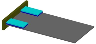
Table 1Geometrical and physical parameters of ACLD/plate system
Aluminum | P-5H | ZN-1 | |||||
0.0008 m | 0.0005 m | 0.001 m | 148.0 | ||||
69 GPa | 74.5 GPa | 0.3 | 12.16 | ||||
0.3 | 0.32 | 789.5 kg/m3 | 810.4 | ||||
2800 kg/m3 | 7450 kg/m3 | 554200 Pa | 896200 | ||||
, | 186×10-12 C/N | 3.960 | 927800 | ||||
65.69 | 761300 | ||||||
2.1. Degrees of freedom and shape functions
The CLD/plate is divided into elements and a two-dimensional integrated element with four nodes shown in Fig. 2 is considered to model the CLD/plate system. Each node has seven degrees of freedom, including the longitudinal displacements and of the constrained layer, the longitudinal displacements , of the base plate, the lateral displacement of the whole structure, and the slopes , of lateral displacement. The displacement of an arbitrary point in an element can be interpolated using the following polynomials:
where the constants are determined in terms of twenty-eight components of the node displacements vector of the th element. The element displacement vector is given by:
where , for 1, 2, 3, 4.
Substituting expressed by the nodes displacements and the nodes coordinates into Eq. (1), the displacement at any location (, ) inside the th element can be described by:
where:
are termed as the shape function, and , are the coordinates of the nodes in the th element coordinates system. Eq. (3) can be rewritten in the matrix form as:
where , , , , , , are called the shape function for , , , , , , .
The deformation relationship of the CLD patches and the base plate is shown in Fig. 3. Then, the displacements in -direction and -direction of the viscoelastic layer (VL) can be formulated as:
Fig. 2The CLD element
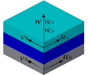
Fig. 3The deformation relationship
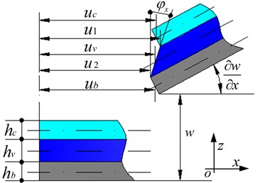
And the shear deformation of the VL can be derived as:
where , and , , denote the thickness of the base plate, the constrained layer and the viscoelastic layer respectively.
Hence, the shape functions for the longitudinal displacements and the shear deformations , of the VEM core can be derived as [4]:
So the displacement vector of the VEM can be expressed as:
2.2. Energies of a CLD/plate system
2.2.1. Potential energies
The potential energies related with the plane stress deformations of the CLD/plate system are expressed as:
where denote the base plate, the constrained layer and the viscoelastic layer, respectively. , are Young’s modulus and Passion’s ratio, and is the thickness for the three layer in the CLD/plate system, respectively. Substituting Eq. (4) into Eq. (10) for base plate and constrained layer, the can be obtained as follows:
where is the elastic coefficient matrix with , , and . So the membrane stiffness matrices for the base plate and the constrained layer can be defined as:
For viscoelatic layer, the shape functions are related with the thicknesses , , , so the is also related with these parameters. To investigate conveniently the characteristics what these parameters have effect on, the from which the , , are factored out is expressed as follows:
where , , , are:
So the membrane stiffness matrix for viscoelastic layer is obtained as:
Furthermore, the potential energies related with the bending deformations of the CLD/plate system are expressed as:
Substituting Eq. (4) into Eq. (15), can be obtained as follows:
where . So the bending stiffness matrices for every layer in the CLD/plate system can be defined as:
For the CLD/plate system, the vibration energy is consumed by the shear deformation of the VEM. The potential energy related with the shear deformations of the VEM is derived as:
where is the shear modulus of the VEM. Substituting Eq. (9) into Eq. (18), the , like the potential energy , can be obtained as follows:
where , , are:
So the shear stiffness matrices for viscoelastic layer is obtained as:
2.2.2. Kinetic energies
The kinetic energy for each layer of the CLD/plate system is expressed as:
where denote the base plate, the constrained layer and the viscoelastic layer, respectively. , are density and the thickness for the three layers in the CLD/plate system, respectively. Substituting Eq. (4) into Eq. (21) for base plate and constrained layer, the can be obtained as follows:
So the element mass matrices for the base plate and the constrained layer can be defined as:
For viscoelatic layer, like the stiffness matrix, the element mass matrix can be defined as:
where , , are:
2.2.3. Work done by the external force
The virtual work done by the external disturbance is:
2.3. Equation of motion
Applying the energy method, the equations of motion for an ACLD element can be written as:
where .
The frequency- or time-dependent behavior of the visco-elastic material is now modeled by using Golla-Hughes-McTavish (GHM) method [15]. In this approach, the shear modulus of VEM is expressed as a series of ‘mini-osillator’ terms in the Laplace domain:
where the constants , and govern the shape of the modulus function over the complex s-domain. A column matrix of dissipation co-ordinates is introduced as follows:
Considering a three-term GHM expression, Eq. (24) can be rewritten as follows:
where each vector and matrix can be expressed as:
where , , , , is a diagonal matrix of the positive eigenvalues of matrix , and is the eigenvectors matrix corresponding to the eigenvalues.
The global equations of motion can be obtained via assembling the element mass and stiffness matrices, and the element force vectors, as follows:
3. Problem formulations
Most real-world search and optimization problems naturally involve multiple objectives. For the optimization problem of the CLD structures, it requires that several trade-off CLD configurations, using which the selected resonance peaks can be decreased simultaneously, can be obtained. Thus, it can be considered as a multi-objective optimization problem. The standard form of the multi-objective optimization problem for CLD/plate can be described as:
where is the vector of the design variables.
3.1. Objective functions
Based on Eq. (30), the state space model of the CLD/plate can be derived as follows:
The complex eigenvalues corresponding to Eq. (32) are expressed as:
where , are the real and imaginary parts of the th complex eigenvalue, respectively, and . Here, the loss factor of the th complex mode are defined as:
Obviously, the loss factor is larger, the vibration of the structure is decayed more quickly, and the efficiency of vibration suppression becomes better. So, the objective functions used in this study can be stated as follows:
3.2. Design variables and optimization strategies
The parameters of viscoelastic material (VEM) and constrained layer material (CLM) and the locations of the CLD patches are significant on the vibration and damping characteristics of CLD structure. So locations of the CLD patches on the base structure and thicknesses of the VEM and CLM are selected as the design variables, i.e.:
where denotes the location of the th CLD which is expressed by the positive integer, and for , is the number of the CLD. and which are expressed by positive continuous real number, are the thicknesses of the VEM and CLM, respectively. and are the number of the thickness variables. Thus, the design variable vector contains different variable type, i.e. it is a hybrid variable vector.
Due to the variable vector containing two different types, two optimization strategies are proposed to optimize the CLD/plate structure as follows:
1) Firstly, the locations of the CLD patches are optimized, and then the optimal thicknesses of VEM and CLM are obtained. That is ‘step-by-step optimization’.
2) The locations, the thicknesses of VEM and CLM, which consists of the hybrid variable vector, are optimized simultaneously. That is “integrated optimization”.
3.3. Constraints
Considering design requirements for the engineering structures, the added weight and the shift of the natural frequencies should be in a limited range. i.e.:
where is the added weight when the CLD patches are pasted on the base structure, and are the feasible minimum and maximum added-mass. and can be calculated as:
where, and are the coefficients, is the number of CLD patches, and are the densities of VEM and CLM, and are the minimums of VEM and CLM, and are the maximums of VEM and CLM, and are the size of the element. and are the natural frequencies of the CLD/plate before and after the optimization procedure is carried out.
4. Multi-objective optimization algorithm-improved NSGA-II
For multi-objective optimization for CLD structure, the relationship between the design variables and the objectives is hard to describe by the use of explicit mathematical equations. Meanwhile, the design variables space composes of two different types of design variables: discrete and continuous. Besides, due to the difficulty of characterizing visco-elastic properties of VEM accurately, that makes the optimization problem more complex. As well known, the traditional optimization strategies, such as linear programming algorithm, are powerful to solve single objective optimization problem described by explicit mathematical equations, but difficult to solve the complex multi-objective problem. However, GA is very useful and powerful to deal with such multi-objective optimization problem. In this paper, the non-dominated sorting genetic algorithm (NSGA-II), which has an excellent robustness, is introduced and improved to solve the hybrid variables multi-objective optimization problem.
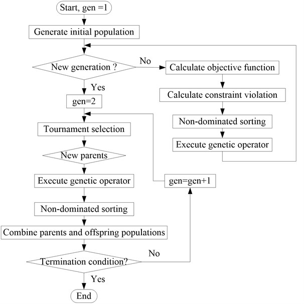
The basic flow chart of the NSGA-II algorithm which is proposed by Deb [16], considering the constrained condition, is employed to carry out the optimization shown in Fig. 2. Some basic ideals are explained as follows:
(1) Chromosome representation. In this investigation, to overcome the ‘Hanming Cliff’ in the binary codes, all the values of the design variables are encoded by decimal code that is different from the original NSGA-II algorithm. For simplicity, the chromosome constructions of hybrid variables, objective function value, constraint violation value, the rank value, the crowding distance, are shown in Fig. 3.
(2) Constraint handling. In the multi-optimization problem, the constraint violation is described as:
In the constraint handling approaches, a tournament selection is employed where two solutions are compared at a time, and the following criteria are always enforced [17]:
a) Any feasible solution is preferred to any infeasible solution.
b) Among two feasible solutions, the one having smaller constraint violation is preferred.
c) Among two infeasible solutions, the one having smaller constraint violation is preferred.
(3) Non-dominated sorting. The constrain-domination condition [18] for any two solutions is described as follows:
If a solution is said to ‘constrain-dominate’ a solution , then any of the following conditions are true:
a) Solutions is feasible and solution is not.
b) Solution and are both infeasible, but solution has a smaller constraint violation.
c) Solution and are feasible and solution dominates solution in the usual sense.
In the non-dominated sorting procedure, for each solution, two entities will be calculated firstly: 1) domination count , the number of solutions which dominate the solution , and 2) , a set of solutions that the solution dominates. Then the following procedure [16] is used to carry out the non-dominated sorting.
Step 1: Find all the solutions with the domination count being zero, and set these solutions in the first non-dominated front. The rank value for these solutions is set to be one.
Step 2: For each solution with , each member of its set is visited and its domination count is reduced by one.
Step 3: In doing so, if for any member , the domination count becomes zero, it will be put in a separate set . These members belong to the second non-domination front. The rank value for these solutions is set to be two.
Step 4: The above procedure is continued with each member of and the third front is identified. And the process continues until all fronts are identified.
(4) Crowding distance. The crowding distance of the th solution (marked with solid circles) in its front which is shown in Fig. 4, is the average side-length of the cuboids (shown by a dashed box). It denotes the diversity distribution of the solution in its front.
Fig. 4Flow chart of the optimization algorithm
(5) The genetic operator
In the standard NSGA-II, simulated binary crossover operator and polynomial mutation operator are served as genetic operators. But they can be used to solve real coded optimization problem. Herein, the new genetic operators are introduced and improved for the special optimization problem of the CLD/plate.
a) The new crossover operator
The Laplace crossover operator which is proposed in [19], is introduced in the NSGA-II to deal with the hybrid/mixed design variables optimization problems. According to the Laplace crossover operator, the two offspring produced by the two parents, , are computed as:
where:
, are uniform random numbers between 0 and 1, is called location parameter, and is termed as scale parameter. For integer design variables, , is usually assigned to be an integer, otherwise, is set to be a positive real value below 1. For smaller value of , offspring are expected to be produced near the parents, and for lager , offspring are likely to be produced far from parents.
Because two or more CLD patches can not be bonded on the same location on the base plate, i.e., for , the procedure of the original crossover operator will be modified. Based on the smallest distance principle, the crossover operator will be carried out for every pair variables denoting the locations of CLD patches in the parent. The procedure is expressed as follows:
Step 1: The crossover operator is carried out for the first pair variables and in the parent and the first two offspring are got as follows:
Step 2: The range and for the second two offspring are updated to:
Step 3: The crossover operator is carried out for the first pair variables and in the parent and the second two offspring are obtained as follows:
If or , then and will be revised as:
Step 4: Step 2 and Step 3 are continued until the crossover operator is carried out for every integer variable pair.
b) The new mutation operator
The power operator which is proposed in [19], is introduced in the NSGA-II as mutation operator to deal with the hybrid/mixed design variables optimization problems. According to the mutaion operator, the offspring produced by the parents, , is generated as:
where , is an uniform random number in the range of 0 to 1, is named as the power distribution index of mutation. , is usually assigned to be a positive integer for integer design variables, otherwise, is set to be a positive real value less than 1. For large values of , more diversity in the solutions is expected, and for small valves of , less perturbance is achieved. , , are lower and upper limits of the th design variable. is a uniformly distributed random number between 0 and 1.
When the mutation operator is carried out for integer variables, the similar procedure like that of the crossover operator is employed.
(6) Truncation for integer variables. After the crossover and mutation operator are performed, the variables denoting the locations of CLD patches are truncated to integer. The rule is described as follows:
a) if is an integer, then , otherwise;
b) is equal to either or each with probability of 0.5, is the integer part of .
5. Optimization results and discussions
5.1. The cantilever CLD/plate
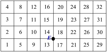
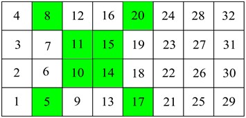
The cantilever CLD/plate which is divided into 8×4 elements, is shown in Fig. 5. The left side of the plate is clamped. The numbers on the element denote the locations for CLD patches which will be bonded on the base plate, as well as the element numbering. The base plate, with the size of 0.2×0.1 m2, is partly treated with CLD treatments. The main physical parameters of the base plate (Aluminum), viscoelastic layer (ZN-1) and piezoelectric layer (P-5H) are listed in Table 1. In the following optimization procedure, the range of thickness is . And the point in Fig. 7 is set to measure the vibration response of the plate.
Fig. 5Chromosome constructions. c denotes the constraint violation value, r denotes the rank value for ith solution, cd denotes the crowding distance of the ith solution
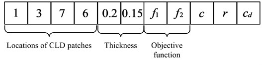
Fig. 6The crowding distance calculation
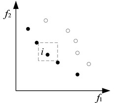
Fig. 7Finite element partition of the CLD/plate
5.2. “Step-by-step optimization” for CLD/plate
“Step-by-step optimization” for CLD/plate is carried out. Firstly optimal locations of CLD patches for taking the first two mode loss factors maximization as the objective functions are obtained by carrying out the multi-objective optimization procedure using the above improved NSGA-II (INSGA-II). The thicknesses of VEM and CLM are the same as that in Table 1. The number of CLD patches is selected as eight. The genetic parameters and are set to be 0.5 and 8.
The Pareto front is shown in Fig. 8. It is observed that the Pareto front is a set of points distributing like a curve because of the discrete design variables, and the first mode loss factor increases with the second mode loss factor decreasing. Four different layouts of CLD patches which are illustrated in Fig. 10 are selected to analyze the effectiveness of vibration suppression. For the layout 1 and layout 7, the CLD patches are placed on the locations where the mode strain energy for the first two modes, is maximum, shown in Fig. 11. The result is consistent with that in reference [5]. The frequency responses of base plate and different layouts of CLD patches are plotted in Fig. 9. It is reasonable to believe that: (1) it is very effective to reduce the first two resonances for all the layouts of CLD patches; (2) layout 1 is more effective for suppressing resonance of the first mode; (3) on the contrary, layout 7 is more feasible to control the vibration induced by the disturbance with the second mode frequency; (4) compared to layout 1 and 7, layout 3 and 5 may be the trade-off configurations for CLD patches to reduce the vibration of the first two modes; (5) especially, for layout 5, the control performance is close to that of the layout 1 for the first mode and is close to that of layout 7 for the second mode; (6) compared with the base structure for which the first two mode frequencies are 16.44 Hz and 70.805 Hz, the natural frequencies for CLD/plate are changed a little, but still in an acceptable range.
Fig. 8The Pareto front for locations of CLD patches optimization
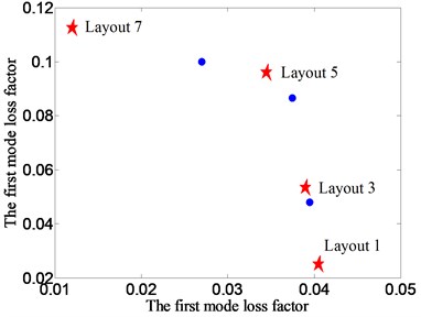
Fig. 9FRFs for different layouts of CLD patches
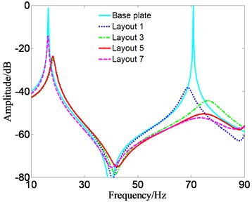
Fig. 10The different Pareto optimal layout for CLD patches
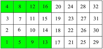
a) Layout 1
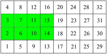
b) Layout 3
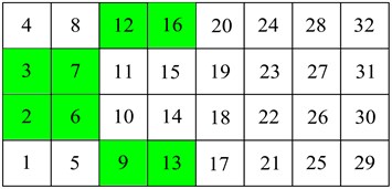
c) Layout 5
d) Layout 7
Then the thicknesses of VEM and CLM for layout 5 are optimized by use of INSGA-II. Here, mass constraint is employed, which is , and the coefficients , . Furthermore, the frequency constraint is added, in which the frequency shift limitation is set to be about 20 % of the original value for the first mode, and about 10 % for the second mode.
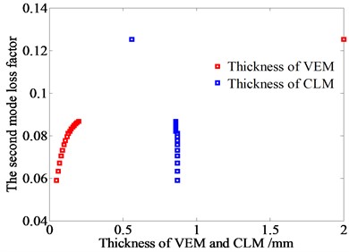
Fig. 12 shows the Pareto front for layout 5 under the two constraints. A series of Pareto optimal configurations of thickness can be obtained when mass constraint is employed, and only a configuration is received when mass and frequency constraints are considered simultaneously. Fig. 13 shows the frequency responses for different configurations of and . Fig. 14 demonstrates the added-mass and frequency shift for different optimal thickness configurations, and Fig. 15 displays the relationship between optimal thickness of VEM/CLM and the first two modes’ loss factor.
Fig. 11Mode strain energy of the first two modes for CLD/plate
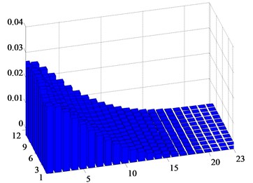
a) Mode 1
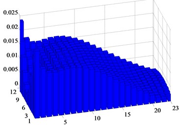
b) Mode 2
Fig. 12Pareto front for laytout 5
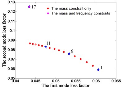
Fig. 13FRF for different Pareto optimal configurations of hv and hc
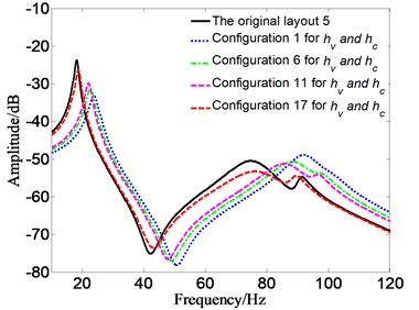
Fig. 14The added-mass and the frequency shift for different optimal configurations
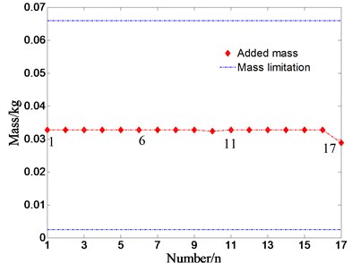
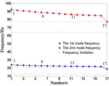
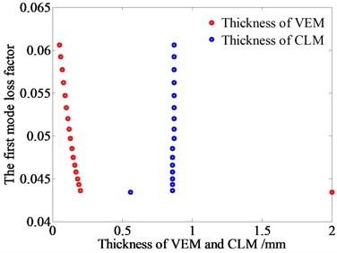
It is apparent that: (1) the mode loss factor is more sensitive to the mode frequency constraint and the first mode loss factor increases with thickness of VEM decreasing, but the second mode loss factor decreases; (2) compared to the original layout 5, the better vibration suppression of the first two modes can be achieved for almost all the configurations of and , regardless of constraint conditions; (3) the added-mass keeps a constant and the mode frequencies exceed the limitations except for configuration 17; (4) thickness of CLM keeps a constant close to 0.9 mm, and thickness of VEM varies from 0.05 mm to 0.2 mm in general; (5) compared Fig. 13 with Fig. 12, there is a tendency that when thickness of CLM keeps a constant, the natural frequency of the CLD/plate increases with thickness of VEM increasing; (6) there is a special configuration for and , ( 2 mm, 0.56 mm), corresponding to configuration 17, in which the maximum second mode loss factor is obtained.
Fig. 15Relationship between thickness of VEM/ VLM and the first two mode loss factor
5.3. Integrated optimization for CLD/plate
The integrated optimization for CLD/plate is carried out. In the procedure, locations of CLD patches and thicknesses of VEM and CLM consist of hybrid variables, and the first two mode loss factors are taken as objective functions. The mass constraint is employed firstly, and then the mass and frequency constraints are considered simultaneously. Optimal variables and objective functions are listed in Table 2 and Table 3. It is very clear that the CLD patches for the first two maximal mode loss factors are bonded on the locations where the mode strain energy is maximal. That is consistent with “step by step optimization”. Fig. 16 displays the Pareto fronts for the two cases. It clearly reveals that the first mode loss factor varies oppositely to the second mode loss factor. A comparison between the fronts shows that the mode loss factor becomes smaller when the frequency constraint is employed, especially for the first mode loss factor. Thus, it can be inferred that the vibration suppression for the first mode is more effective when the mass constraint is considered exclusively.
Fig. 16Pareto fronts for hybrid variables
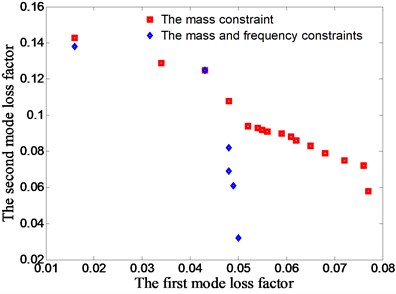
Fig. 17Relationship of hv/hc and mode loss factor
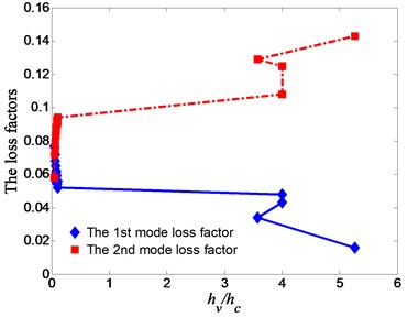
For consideration of the mass constraint, the locations of CLD patches described in number 4 of Table 2 may be a preferred trade-off configuration. Furthermore, Fig. 17 reveals that when the remains around 0.05-0.1, the performance for controlling the first mode of vibration is better and when the remains a larger value (greater than 3.6), the performance for controlling the second mode of vibration is better. Considering the mass and frequency constraints simultaneously, it can be seen from Table 3 that thickness of VEM is up to the upper limitation. And the first mode loss factor varies very little except configuration 6, otherwise the second mode loss factor has a large range. So it can be inferred that for vibration control of the first mode, the variation is not obvious except that of configuration 6, but that is contrary for the second mode. That is verified in Fig. 18. Fig. 19 and Fig. 20 display that the added-mass and the mode frequency variation for the above two cases. A comparison between the two cases shows that for the first case, although there will be more configurations of CLD patches and a large mode loss factors range, it will have a larger added-mass and a larger mode frequency variation. Thus, it can be referred the second case may be a better selection in real-world optimization problem.
Table 2The Pareto solutions and objective functions with mass constraint only
Number | Locations of CLD patches | (mm) | (mm) | 1st loss factor | 2nd loss factor |
1 | 1, 4, 5, 8, 9, 12, 13, 16 | 0.05 | 0. 98 | 0.077 | 0.058 |
2 | 2, 3, 6, 7, 10, 11, 14, 15 | 0.05 | 0. 97 | 0.076 | 0.072 |
3 | 2, 3, 6, 7, 10, 11, 14, 15 | 0.05 | 0. 8 | 0.072 | 0.075 |
4 | 2, 3, 6, 7, 10, 11, 13, 16 | 0.06 | 0.99 | 0.068 | 0.079 |
5 | 2, 3, 6, 7, 10, 11, 13, 16 | 0.07 | 0.94 | 0.065 | 0.083 |
6 | 2, 3, 6, 7, 10, 11, 13, 16 | 0. 08 | 0.94 | 0.062 | 0.086 |
7 | 2, 3, 6, 7, 10, 11,13, 16 | 0. 09 | 1.08 | 0.061 | 0.088 |
8 | 2, 3, 6, 7, 10, 11,13, 16 | 0.10 | 1.08 | 0.059 | 0.090 |
9 | 2, 3, 6, 7, 10, 11,13, 16 | 0.11 | 1.01 | 0.056 | 0.091 |
10 | 2, 3, 6, 7, 10, 11,13, 16 | 0.10 | 1.14 | 0.055 | 0.092 |
11 | 2, 3, 6, 7, 10, 11,13, 16 | 0.11 | 1.14 | 0.054 | 0.093 |
12 | 2, 3, 6, 7, 10, 11,13, 16 | 0.12 | 1.11 | 0.052 | 0.094 |
13 | 2, 3, 6, 7, 9, 12, 14, 15 | 2.00 | 0.50 | 0.048 | 0.108 |
14 | 2, 3, 6, 7, 9, 12, 13, 16 | 2.00 | 0.50 | 0.043 | 0.125 |
15 | 1, 4, 6, 7, 10, 11, 13, 16 | 2.00 | 0.56 | 0.034 | 0.129 |
16 | 5, 8,10,11, 14, 15, 17, 20 | 2.00 | 0.38 | 0.016 | 0.143 |
Table 3The Pareto solutions and objective functions with mass and frequency constraints
Number | Locations of CLD patches | (mm) | (mm) | 1st loss factor | 2nd loss factor |
1 | 1, 4, 5, 8, 9, 12, 13, 16 | 2.00 | 0. 45 | 0.050 | 0.032 |
2 | 1, 4, 5, 8, 9, 12, 14, 15 | 2.00 | 0. 49 | 0.049 | 0.061 |
3 | 2, 3, 6, 7, 10, 11, 14, 15 | 2.00 | 0. 48 | 0.048 | 0.068 |
4 | 2, 3, 5, 8, 9, 12, 14, 15 | 2.00 | 0.52 | 0.048 | 0.082 |
5 | 2, 3, 6, 7, 9, 12, 13, 16 | 2.00 | 0.54 | 0.043 | 0.125 |
6 | 5, 8,10,11, 14, 15, 17, 20 | 2.00 | 0.27 | 0.016 | 0.138 |
Comparison between ‘step-by-step optimization’ and ‘integrated optimization’ shows that: (1) locations of CLD patches for the two maximal mode loss factors are the same; (2) more optimal CLD patches configurations and larger range of loss factors are obtained using “integrated optimization”, and it means that more feasible configurations of CLD patches can be in a selection list; (3) for controlling the first mode of vibration, the should be a smaller value, and for controlling the second mode of vibration, the should be a larger one without considering the mode frequency variation; (4) the will be up to the upper limitation with considering the added-mass and mode frequency variation simultaneously.
Fig. 18FRF for mass and frequency constraints
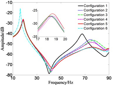
Fig. 19The added-mass for the two cases
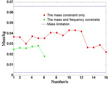
Fig. 20Mode frequency variations for different constraints
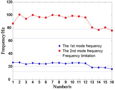
a) The mass constraint only
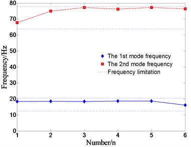
b) The mass and frequency constraints
5.4. Discussions of genetic parameters
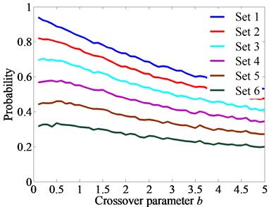
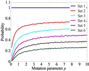
Fig. 21 show the relationships between parameters , and the variables probability. And the probability denotes that the variables are located in the decreasing ranges (from set 1 to set 6) when the genetic operators are carried out for 10000 times. Based on Fig. 21, 0.5 and 8 are selected in the precious optimization procedure.
Fig. 21The relationship between parameters b, p and the variables probability
a)
b)
For simplicity, taking the above integrated optimization with mass and frequency constraints as an example, the effect that the crossover probability and mutation probability have on the optimization procedure are analyzed. When crossover probability decreasing (from 0.95 to 0.5) and mutation probability increasing (from 0.05 to 0.5), the convergence procedures are obtained in Fig. 22. It can be seen that the optimization procedure converges well when mutation probabilities are smaller, and fluctuations appear when mutation probabilities are larger. It is noted that the pattern is obtained while optimization procedures for every set are carried out for many times. Besides, when the mutation probabilities are too small, such as 0.05, the best Pareto solutions cannot always be obtained.
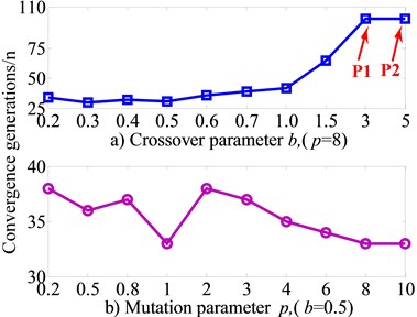
When crossover probability is 0.9 and mutation probability is 0.1, the relationships between convergence generations and parameters , are discussed, shown in Fig. 23. It is very clearly that: 1) when crossover parameter is smaller than 1, convergence generations vary tinily, 2) when it is more than 1, convergence generation increases greatly, 3) when it is larger than 3 (point P1), the convergence still cannot be obtained while 100 generations are carried out, 4) when mutation parameter increases, the convergence generations vary tinily due to smaller mutation probability. It is also noted that the pattern is obtained while optimization procedures for every set are carried out many times.
Fig. 22The optimization procedure with different crossover and mutation probabilities
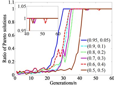
Fig. 23Relationships between b, p and convergence generations
6. Conclusions
In this paper, the multi-objective optimization model of CLD/plate is established based on finite element method (FEM) in conjunction with Golla-Hughes-McTavish (GHM) method. The objectives are to maximize the first two mode loss factors and the design variables are locations of the CLD patches and thicknesses of viscoelastic material (VEM) and constrained layer material (CLM) which consist of hybrid variables. The improved non-dominated genetic algorithm (INSGA-II) is proposed and two different optimization strategies are employed. As results of the optimization, reasonable pareto solutions about CLD configurations are successfully obtained. It is shown that the INSGA-II is very suitable to the multi-objective optimization problem and the optimization strategies are applicable for the CLD treatments structure optimization.
The vibration characteristics of the CLD/plate based on Pareto solutions are discussed. The different reasonable configurations of CLD treatments can be obtained except for some special cases by use of different optimization strategies. The effectiveness of vibration control for different modes depends highly on the ratio of and locations of CLD treatments on the Pareto fronts. Furthermore, the optimal configurations of CLD treatments are also sensitive to constraint condition, and different tendencies of parameters of VEM and CLM can be obtained under different constraint conditions. Therefore, the multi-objective optimization will supply different trade-off optimal configurations for CLD treatments structure under different vibration control objective and constraint conditions.
Besides, the influence of genetic parameters on optimization procedure is also discussed. The crossover parameter and mutation parameter can be selected in a large range. Fluctuations in optimization procedure will happen when a larger mutation probability is employed, and premature may occur when a smaller mutation is selected. The crossover parameter has an obvious effect on the optimization procedure.
References
-
Ray M. C., Baz A. Control of nonlinear vibration of beams using active constrained layer damping. Journal of Vibration and Control, Vol. 7, Issue 4, 2001, p. 539-549.
-
Kumar Navin, Singh S. P. Vibration and damping characteristics of beams with active constrained layer treatments under parametric variations. Materials and Design, Vol. 30, Issue 10, 2009, p. 4162-4174.
-
Vasques C. M. A., Dias Rodrigues J. Combined feedback/feedforward active control of vibration of beams with ACLD treatments: Numerical simulation. Computers and Structures, Vol. 86, Issue 3-5, 2008, p. 292-306.
-
Ling Zheng, Dongdong Zhang, Yi Wang Vibration and damping characteristics of cylindrical shells with active constrained layer damping treatments. Smart Material and Structure, Vol. 20, Issue 2, 2011, p. 025008.
-
Ro J., Baz A. Optimum placement and control of active constrained layer damping using mode strain energy approach. Journal of Vibration and Control, Vol. 8, Issue 6, 2002, p. 861-876.
-
Mantena P. R., Ronald F. Gibson, Shwilong J. Hwang Optimal constrained viscoelastic tape lengths for maximizing damping in laminated composites. AIAA Journal, Vol. 29, Issue 10, 1991, p. 1678-1685.
-
Kodiyamalam S., Molnar J. Optimization of constrained viscoelastic damping treatments for passive vibration control. Proceedings of 33RD Structures, Structural Dynamics and Materials Conference, 1992.
-
Marcelin J. L., Trompette P., Smati A. Optimal constrained layer damping with partial coverage. Finite Elements in Analysis and Design, Vol. 12, 1991, p. 273-280.
-
Kung S. W., Singh R. Development of approximate methods for the analysis of patch damping design concept. Journal of Sound and Vibration, Vol. 219, Issue 5, 1999, p. 785-812.
-
Zheng H., Cai C., Pau G. S. H. A comparative study on optimization of constrained layer damping treatment for structural vibration control. Thin-Walled Structures, Vol. 44, Issue 8, 2006, p. 886-896.
-
Al-Ajmi M., Boursili R. Optimum design of segmented passive constrained layer damping treatment through genetic algorithms. Mechanics of Advanced Materials and Structures, Vol. 15, Issue 1, 2008, p. 250-257.
-
Zheng Ling, Xie Ronglu, Wang Yi Optimal placement of constrained damping material in structures based on optimality criteria. Journal of Vibration and Shock, Vol. 11, 2010, p. 156-159, 179, 259-260.
-
Yinong Li, Ronglu Xie, Ling Zheng Topology optimization for constrained layer damping material in structures using ESO method. Journal of Chongqing University, Vol. 8, 2010, p. 1-6.
-
Lepoittevin Grégoire, Kress Gerald Optimization of segmented constrained layer damping with mathematical programming using strain energy analysis and mode data. Materials and Design, Vol. 31, Issue 1, 2010, p. 12-24.
-
McTavish D. J., HughesP. C. Modeling of linear viscoelastic space structures. American Society of Mechanical Engineers, Journal of Vibration and Acoustics, Vol. 115, 1993, p. 103-110.
-
Deb K., Pratap A., Agarwal S. A fast and elitist multi-objective genetic algorithm: NSGA-II. Evolutionary Computation, Vol. 6, Issue 2, 2002, p. 182-197.
-
Deb Kalyanmoy An efficient constraint handling method for genetic algorithms. Computer Methods in Applied Mechanics and Engineering, Vol. 186, Issue 2-4, 2000, p. 311-338.
-
Deb Kalyanmoy Multi-objective Optimization using Evolutionary Algorithms. John Wiley and Sons Inc., New York, 2008.
-
Deep Kusum, Singh Krishna Pratap, Kansal M. L., Mohan C. A real coded genetic algorithm for solving integer and mixed integer optimization problems. Applied Mathematics and Computation, Vol. 212, Issue 2, 2009, p. 505-518.
About this article

This work was supported by Nature Science Foundation of China (No. 50775225), Research Foundation of State Key Laboratory of Mechanical Transmission (No. 0301002109165). These financial supports are gratefully acknowledged.
