Investigation on the aerodynamic characteristics of a rocket-target for the system “Stinger”

1. Introduction

The geometrical and design parameters and the exterior ballistics characteristics of a rocket are usually estimated for a particular rocket design. The range of rocket’s velocities can be rather wide. The present design required developing a rocket-target for the system “Stinger” which is 5 meters in length and 0.4 meters in diameter, at a velocity range below 250 m/s. Several possible nose shapes are suitable in this case, such as various ogive, conical or elliptical shapes [1, 2]. It is known that various aerodynamic characteristics have a great influence on the exterior ballistics of the rocket, however, the drag force and drag coefficient are the most important parameters necessary for the investigation of exterior ballistics.

Computational fluid dynamic (CFD) techniques to calculate the aerodynamic coefficients of many complex geometry and complex flow phenomena were recently demonstrated [3, 4]. CFD is suitable to use at conceptual design stage of the aerodynamic configurations as it is able to get aerodynamic characteristics from more configurations than wind tunnel testing. Therefore, CFD methods are widely used in order to predict aerodynamic characteristics of rockets during various development stages [5-7].

The main objective of this paper is to identify an optimal configuration of a nose shape by a CFD simulation.

2. Mathematical background of flow simulation

The airflow around the rocket was modeled using the commercial finite element software ANSYS CFX. The set of equations solved by ANSYS CFX are the Reynolds averaged equations given below [8].

where $\rho$ is the density, $U$ is the vector of velocity, $p$ is the pressure, $S_M$ is the momentum source, $\tau$ is the molecular stress tensor (including both normal and shear components of the stress) and $\rho \overline{u_i{u}_j}$ are the Reynolds stresses.

The Reynolds stresses need to be modeled by additional equations of known quantities in order to achieve “closure”. The equations used to close the system define the type of turbulence model [8].

In this study the shear stress transport (SST) turbulence model was applied which is the most suitable for aeronautics flows with strong adverse pressure gradients and separation. The model (written in conservation form) is given by the following [9]:

where $k$ is the turbulence kinetic energy, $\omega$ is the turbulence frequency, ${\mu }_t$ is the turbulent viscosity. Blending function $F_1$ is defined by:

where $y$ is the distance from the field point to the nearest wall:

$F_1$ is equal to zero away from the surface ($k$-$\epsilon$ model), and switches over to one inside the boundary layer ($k$-$\omega$ model).

The turbulent eddy viscosity is defined as follows:

where $v_t={\mu }_y/\rho$, $S$ is the invariant measure of the strain rate and $F_2$ is a second blending function:

A production limiter is used in the SST model to prevent the build-up of turbulence in stagnation regions:

The constants for the SST model are: $a_1=$0.31, ${\beta }^{*}=$ 0.09, ${\mathrm{\alpha }}_1=\mathrm{}$5/9, ${\beta }_1=\mathrm{}$3/40, ${\sigma }_{k1}=\mathrm{}$0.85, ${\sigma }_{\omega 1}=\mathrm{}$0.5, ${\alpha }_2=\mathrm{}$0.44, ${\beta }_2=\mathrm{}$0.0828, ${\sigma }_{k2}=$ 1, ${\sigma }_{\omega 2}=\mathrm{}$0.856.

The total energy heat transfer model was used in this study which models the transport of enthalpy and includes kinetic energy effects. The total energy equation [8]:

where $\lambda$ is thermal conductivity, $T$ is temperature, $S_E$ is the energy source $h_{tot}$ is the total enthalpy, related to the static enthalpy $h\left(T,p\right)$ by:

3. Computational model of the airflow simulation

Several possible nose shapes (ogive, conical, 0.5 power and elliptical) for the rocket-target were investigated in respect of aerodynamic characteristics (Fig. 1). The overall dimensions of the rocket are 0.4 m in diameter and 5.6 m in length and the overall dimension between the fins is 1.2 m. The length of the nose is 0.4 m (the same for all the configurations).

Fig. 1Rockets with different shape nose cones

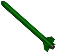
a) Ogive

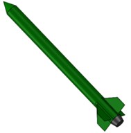
b) Conical

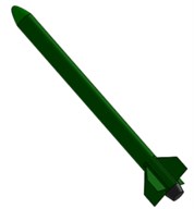
c) 0.5 power

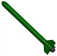
d) Elliptical

Three dimensional models of computational domains for the rockets were produced in SolidWorks and imported into ANSYS CFX. Computational numerical finite element models for a numerical simulation of airflow around the rockets were generated in ANSYS CFX software. Only a half of each model is discretized with a symmetry boundary condition in order to save computational time. A rectangular fluid domain was placed around the rocket, in order to limit the fluid domain where the CFD simulation is carried out. The limit upstream the body was located at a distance of 3 rocket’s lengths and the limit downstream the body was located at a distance of 5 rocket’s lengths, whereas the lateral boundaries were placed at a distance of about 35 diameters (~2.5 rocket’s lengths).

Fig. 2Computational grid cuts at different locations

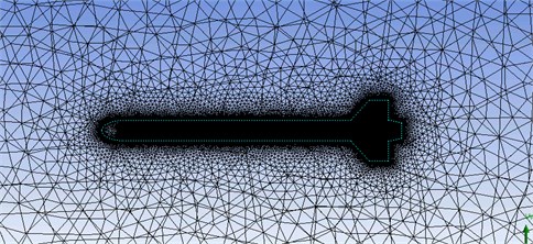
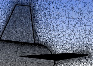
An unstructured computational grid was generated inside this fluid volume. The grid is of hybrid type, i.e. made up of prismatic elements in the viscous region located in close proximity of the body, whereas tetrahedral elements were used to fill the remaining fluid volume. After a mesh sensitivity analysis, the maximum size of tetrahedral elements in the grid was set to 13.5 m and the minimum size was 7.5 mm. 20 layers of prism elements were created on the surface of the rocket with the maximum thickness of 15 mm and the growth rate 1.2. On the surface of the rocket the grid was made distinctly denser, the size of prism elements was set to 3.75 mm. The grid contains an overall size of ~7.18 million elements including ~3.5 million prism elements (Fig. 2).

The assigned range of velocity was between 0.3 and 0.8 Mach number. The standard atmosphere values of all the other thermodynamic variables at sea level were used as input flow conditions in the computations, that is a freestream static temperature of 15 °C and a freestream static pressure of 101327 Pa. The surface of the rocket was defined as a non-slippery smooth wall. The outside walls of the computational domain (the lateral boundaries) were defined as free slip walls.

The analysis was carried out considering the compressible formulation of the Navier-Stokes equation system.

4. Results of the airflow simulation

Results of the simulation of the airflow around the rockets were obtained. The pressure distribution at the surface of the rocket and the cross-section plane is presented in Fig. 3. Velocity streamlines for the rockets at 0.8 Mach number are shown in Fig. 4.

Fig. 3Pressure on the cross-section plane and the rocket surface, under M= 0.8

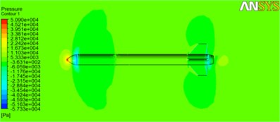
a) Ogive

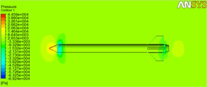
b) Conical

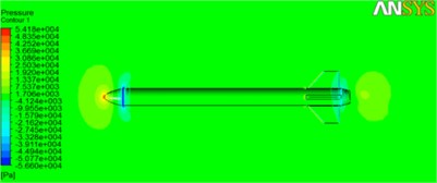
c) 0.5 power

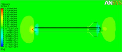
d) Elliptical

Fig. 4Velocity streamlines on the cross-section plane, under M= 0.8

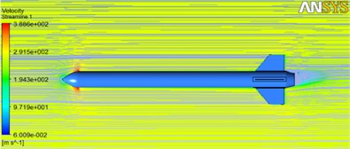
a) Ogive

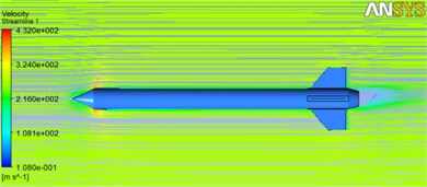
b) Conical

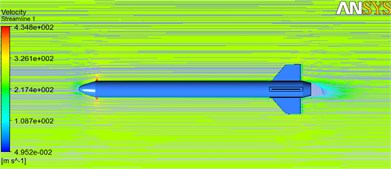
c) 0.5 power

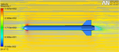
d) Elliptical

The drag coefficient of the rockets was calculated by the following expression [10]:

where $F_d$ is the drag force, obtained from the simulation results; $\rho$ is the air density; $U$ is the velocity of airflow; $A$ is the reference area.

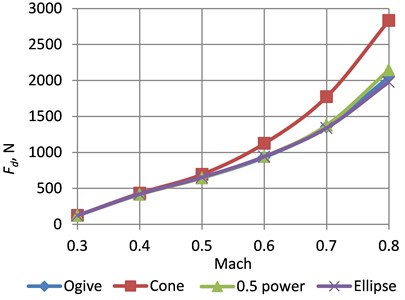
Dependences of the drag force on Mach number for different cones of the rockets is shown in Fig. 5. The highest drag force was for the rocket with the conical nose in all velocity ranges. The simulation showed that the drag force of the rocket with the ogive, conical and elliptical nose shapes is very similar. In the range of 0.3…0.6 Mach number, the lowest drag force is with the ogive nose, then follow the 0.5 power nose and the elliptical nose. In the range of 0.6...0.8 Mach number, the lowest drag force is with the elliptical nose, then follow the ogive nose and the 0.5 power nose. Accordingly, these tendencies reflect on the drag coefficient (Fig. 6).

Fig. 5Dependences of the drag force on Mach number for different cones of the rockets

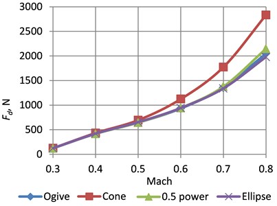
Fig. 6Dependences of the drag coefficient on Mach number for different cones of the rockets

The drag coefficient of the rocket with the ogive, conical and elliptical nose shapes is very close and, in the range of 0.3…0.6 Mach number, it varies from approximately 0.272 (ogive) to 0.353 (0.5 power). As for the conical nose shape, the drag coefficient varies from 0.286 to 0.466 in the same Mach number range.

Since the elliptical nose shape gives the lowest drag force at 0.8 Mach, this shape was selected for further development of the rocket-target.

5. Conclusions

A simulation of the airflow around rockets with different nose shapes is carried out and pressure contours, airflow streamlines, drag force and drag coefficient dependencies on the rocket’s velocity are obtained.

The simulation showed that the highest drag force was for the rocket with the conical nose in all velocity ranges. It is seen, that the drag force of the rocket with the ogive, conical and elliptical nose shapes is very similar. In the range of 0.3…0.6 Mach number, the lowest drag force is with the ogive nose, then follow the 0.5 power nose and the elliptical nose. In the range of 0.6…0.8 Mach number, the lowest drag force is with the elliptical nose, then follow the ogive nose and the 0.5 power nose. Accordingly, these tendencies reflect on the drag coefficient.

The drag coefficient of the rocket with the ogive, conical and elliptical nose shapes is very close and, in the range of 0.3…0.6 Mach number, it varies from approximately 0.272 (ogive) to 0.353 (0.5 power). As for the conical nose shape, the drag coefficient varies from 0.286 to 0.466 in the same Mach number range.

Since the elliptical nose shape gives the lowest drag force at 0.8 Mach, this shape was selected for further development of the rocket-target.