Abstract
Healthy status monitoring of train bearing online is very meaningful work. But as traditional diagnosis system does, performing Fourier spectrum with the datum from more than 200 bearings in a marshalling train is an enormous challenge. Here a healthy status monitoring system of train rolling bearing based on Sparse Fast Fourier Transform (SFFT) is proposed. The monitoring system consists two sequential parts. First, extract fault features based on SFFT spectrum and other time-domain parameters. According to train bearing working environment, altogether 7 fault features are extracted in this paper. Another part is constructing a classifier based on BP neural network. Experimental results show that the system proposed here achieves gratifying results comparing with traditional fault diagnosis system
1. Introduction
Rolling bearings are the key components of trains, whose operating state directly influences the safety of running trains. A real time and effective online diagnosis system of trains rolling bearing could replace time-based maintenance and fault-based maintenance which is currently widely adopted with condition based maintenance. It will not only improve the safety of the operating of traffic transportation, but also greatly lower the cost of train operation. In the field of bearing healthy monitoring system, the method of frequency spectrum analysis of monitoring signals is a sharp weapon to find the failure bearing. However, Fourier transform has a very computational complexity. Even butterfly based Fast Fourier Transform (FFT) also involves operations. There is a large amount of bearings in a marshalling train, such as the CH3-380BL, which contains 184 axle-box bearings and 32 motor bearing. It needs very high hardware cost to analyze bearing health status online if traditional Fast Fourier Transform is used as frequency spectrum analysis tool.
According to the sparse property of the output of the Discrete Fourier Transform (DFT), Haitham Hassanieh et al proposed Sparse Fast Fourier Transform (SFFT) in 2012 [1]. The Fourier transform based on this method can efficiently reduce the runtime cost to and streams of data can be processed 10 to 100 times faster than was possible with the FFT when the sparsity degree ranges in a low sparse scope [2].
In this paper, a healthy status monitoring system of train bearing based on SFFT is proposed. This system can highly improve computation speed while fault diagnosis accuracy just as high as the system based on traditional FFT. The rest of this paper is organized as follows. Firstly, the SFFT algorithm and numerical method are introduced. Secondly, fault features extraction methods, construction of diagnosis system and the effectiveness of the train rolling bearing diagnosis system are provided. And then the conclusion of this paper is given in the end.
2. Sparse fast Fourier transform
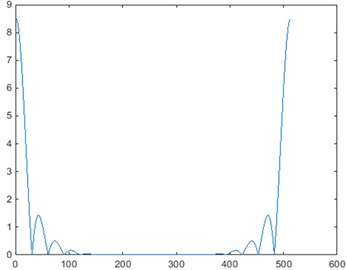
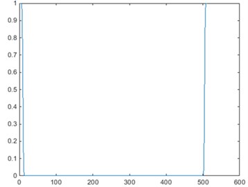
In time domain, given a signal with a -sparse frequency-domain signal . SFFT is a probabilistic algorithm which computes non-zero frequency coefficients that can be reconstructed in a certain probability. The algorithm hashes the Fourier coefficients into bins with n-dimension filter vector which is achieved by convolving a Gaussian function with a box-car function (see Fig. 1). It is convenient to locate and estimate coefficients on account of frequency signal being sparse and only one “large” coefficient probably can be located in every passing region [3].
Fig. 1Filters in time domain and frequency domain: a) Filter G, b) its Fourier Transform G^
a) Filter
b) Filter
2.1. Algorithm
SFFT output satisfies the following guarantee [4]:
where is constant and is an accuracy parameter, is the -sparse vector minimizing .
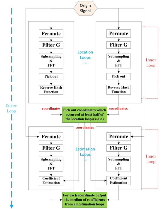
The main idea of SFFT [5] is shown below and a flow diagram is seen in Fig. 2:
1) Run location loops times and return sets of coordinates , ,…, .
2) Count every found coordinate , of which the occurrences are added up to the number : .
3) Retain the coordinates that appeared at least half of the location loops .
4) On the set , operate a number of estimation loops and return sets of frequency coefficients .
5) Estimate every frequency coefficient as where respectively take the median in real and imaginary part.
2.1.1. Location loops
With random parameter invertible mod and , permute the input vector in time: .
Apply a filter with a flat window function , exact a subset of dimensional signal, compute the filtered and permuted vector .
Compute with for , where divides . Here can be computed as the -dimensional DFT of , where for .
Only retain coordinates of maximum magnitude in and form passing regions by interval width . Those are the bins where the non-negligible coefficients were hashed to.
The first 3 steps describe a hash function which maps each of the coordinates of the input signal to one of bins. Here is defined as , which has to be reversed for the coordinates in . One location loop’s output is the set of coordinates mapping to one of the bins in : .
2.1.2. Estimation loops
The function of estimation loops, whose implementation is similar to location loops’, is to reconstruct the exact coefficient values by the given coordinates set .
The first 3 steps share the same ones to location loops’.
Given a set of coordinates , estimate as .
Fig. 2A flow diagram of SFFT
2.2. Implementation of SFFT
Randomly generate a group of signals with the length 512. Permuting in time domain with the permutation causes change in the frequency signal (only keep half of frequency domain), See Figs. 3, 4.
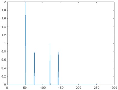
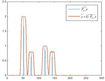
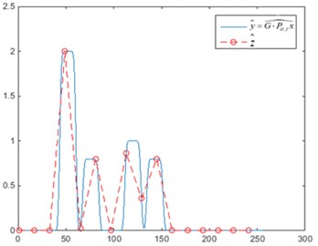
Set 4, 16, compute the time domain signal , of which the spectrum is large around the large coordinates of , such as Fig. 5(a). Next compute , which is the rate subsampling of as plotted in Fig. 5(b), where red pots refer to data points which perform FFT after subsampling.
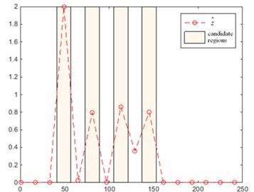
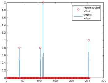
During estimation loops, the algorithm estimates based on the value of the nearest coordinate in . During location loops, the algorithm chooses the largest coordinates of , and selects the elements closest to those coordinates mapped the candidate interval as Fig. 5(c). It outputs the set of original signals of those elements. At this point, the inner loop ends. Finally combining the outer loop, location and value of large coefficient can be obtained in original signal spectrum as Fig. 5(d).
Fig. 3Permutation Pσ,τx of time-domain signal x (σ= 125, τ= 207)
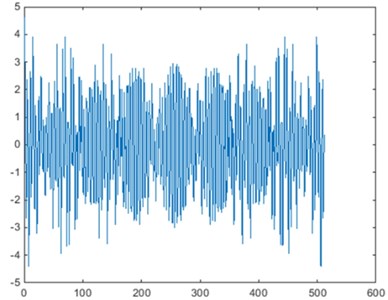
a) Original signal
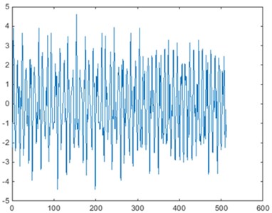
b) Permuted signal
Fig. 4Permutation P^σ,τx of frequency-domain signal x^ (σ=125, τ=207)
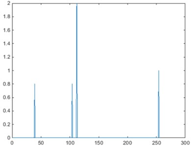
a) Original signal
b) Permuted signal
2.3. Compare SFFT with FFT
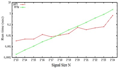
To evaluate the performance of SFFT, this paper compares SFFT with FFTW [6,7] from two aspects. Currently, FFTW is the fastest public implementation for computing the Discrete Fourier Transform and its computational complexity is .
Fix the sparsity parameter 50 and respectively perform SFFT as well as FFT several times. The runtime of the compared algorithms for different signal sizes is plotted in Fig. 6(a). The figure indicates that for signal sizes 10000067108864, SFFT is faster than FFT at 50, which proves the superiority of SFFT over FFT when processing enormous data.
Fix the data size 222 and respectively perform SFFT as well as FFT several times. The runtime of the compared algorithms for different sparsity parameter is plotted in Fig. 6(b). The figure indicates that SFFT runs faster than FFT when ranges in certain sparse scope, that is to say, we can use less data points to realize better fast algorithm.
Fig. 5An example of signal permutation during inner loop and outer loop
a) Convolved signal
b) Subsampling and FFT
c) Estimate passing regions
d) Final result
Fig. 6Contrast result
a) Run time vs signal size (50)
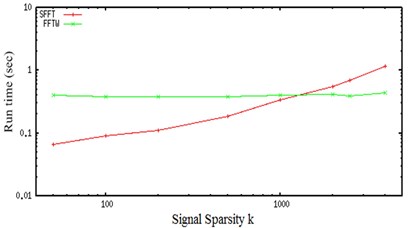
b) Run time vs sparsity (222))
3. Application of SFFT in fault diagnosis system of train rolling bearing
3.1. Fault feature frequencies of rolling bearing
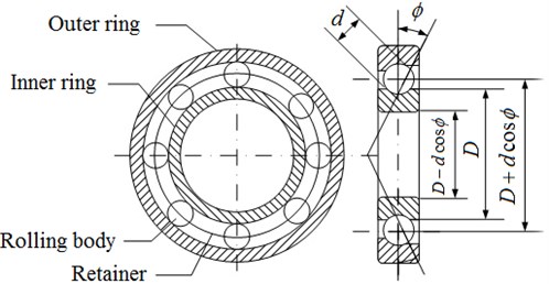
It’s very known that the bearing has four fault feature frequencies, corresponding to outer ring failure (), inner ring failure (), rolling body failure () and retainer failure () [8]. These four kinds of fault feature frequencies are defined as Eqs. (2)-(5):
where is relative rotational frequency between inner ring and outer ring, is the number of rolling body, is the diameter of rolling body, is the pitch diameter of rolling bearing and is contact angle (Fig. 7).
The datum used in this paper come from trains bearing testing table. The corresponding bearing parameters are 29.83 Hz, 9, 0.00794 m, 0.03904 m, 0 rad. Then the four kinds of fault frequencies can be calculated as 106.93 Hz, 161.54 Hz, 128.68 Hz, 11.88 Hz respectively.
Fig. 7Bearing structure
3.2. Fault features extraction for rolling bearing
The validity of fault features has decisive influence on the fault diagnosis system. Another paper of authors Li et al. [9] has verified that amplitude ratios in frequency domain and kurtosis factor, crest factor, clearance factor, impulse factor, shape factor in time domain have good performance on fault diagnosis for train bearing operating in complex environment. In this paper, these features are also adopted to test the proposed method.
3.2.1. Feature in frequency domain
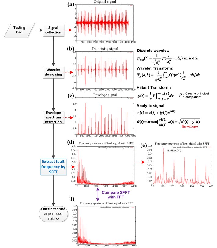
The feature extraction process is shown in Fig. 8. It contains vibration signal analysis with wavelet de-noising [10], envelope spectrum extraction [11] and SFFT.
In this paper, outer ring is taken as the example to test the proposed method. Fig. 8(d) is the spectrogram of the envelope signal of outer ring after SFFT. Fig. 8(e) is the first 600 Hz spectrogram in Fig. 8(d). It can be seen that the amplitude is the largest at 111.33 Hz and the energy is concentrated nearby, so this fault is estimated to be part of outer ring according to Eq. (2). Fig. 8(f) is spectrogram of envelope signal of outer ring performing the traditional FFT. Comparing Fig. 8(d) with Fig. 8(f), it can be seen that the spectrogram tendency of SFFT approximately keeps the same as FFT’s and verifies the validity of SFFT on fault feature extraction.
Feature amplitude ratios are defined as the ratios between the amplitude of outer or inner ring fault frequency, and the amplitude of rolling body fault frequency. In this paper, feature amplitude ratios are extracted on the basis of envelope signal after SFFT, showed in Fig. 8(d). Two feature amplitude ratios are listed as below:
where is the amplitude of fault feature frequency.
Respectively 20 groups of data samples under normal bearing, fault on outer ring, inner ring and rolling body are adopted. Then the fault feature amplitude ratios of every sample are computed by Eqs. (6), (7). Table 1 is one group of the feature amplitude ratios which is selected randomly.
Fig. 8Flow diagram for fault feature extraction of rolling bearing
It can be seen from Table 1, when bearing fault appears on outer ring, is a notable large value while is notably small. When bearing fault appears on inner ring, is a notable small value while is notably large. When fault appears on rolling body or bearing is normal, and are relatively steady but also can be distinguished obviously. Therefore, selecting feature amplitude ratio as the input vector of bearing fault classifier is effective.
Table 1Extract feature amplitude ratios
Type | Normal | Outer ring fault | Inner ring fault | Rolling body fault |
1.2308 | 6.6330 | 0.5456 | 0.0262 | |
0.6739 | 0.1286 | 10.9076 | 0.5529 |
3.2.2. Feature in time domain
This paper chooses 5 parameters as feature extraction in time domain.
Kurtosis factor:
Crest factor:
Clearance factor:
Impulse factor:
Shape factor:
where is root-mean-square value, is root-mean-square amplitude, is absolute average amplitude.
Compute feature parameters in time domain by Eqs. (8)-(12) under 4 kinds of healthy states. The parameters listed in Table 2 are selected randomly from the five feature parameters groups under 4 healthy states respectively. It can be seen that these feature parameters have obvious differences and can effectively distinguish the various fault types.
Table 2One group of feature parameters of time domain in each state
Type | Kurtosis factor | Crest factor | Clearance factor | Impulse factor | Shape factor |
Normal | 3.1860 | 3.9954 | 6.1325 | 5.1177 | 1.2809 |
Fault on outer ring | 17.0284 | 7.6012 | 50.9267 | 19.6712 | 2.5879 |
Fault on inner ring | 28.1688 | 11.3817 | 49.2685 | 27.3709 | 2.4048 |
Fault on rolling body | 4.4376 | 3.8421 | 5.3252 | 4.6493 | 1.2101 |
3.3. Fault diagnosis of rolling bearing
An appropriate fault classifier is needed to be designed for fault diagnosis. There are several kinds of classifiers, of which Artificial Neural Network (ANN) is a highly interconnected network of a large number of processing elements called neurons. It quickly computes a large number of operations by parallel distributed processing [12]. Comparing with decision trees, Logistic Regression (LR) [13] model, ANN can better deal with ordered attributes in most cases [14] and approximate any complex nonlinear relationship and complicatedly partition feature space [15]. ANN is proved to be a powerful data-driven, self-adaptive computational tool which can accurately obtain nonlinear and complex underlying characteristics of physical process [16] and is widely used in fault diagnosing.
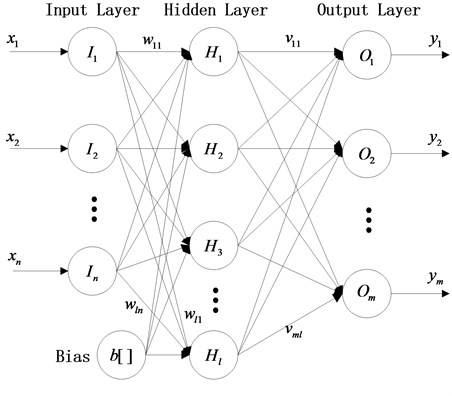
ANN attains knowledge about a problem by being trained with known examples. If the network is trained appropriately, it can be effectively used to solve some ‘unknown’ or ‘untrained’ instances of the problem [17]. ANN is constituted by multiple layers: an input layer, hidden layer (s) and an output layer. In each layer, neurons act as processing elements. Biases are added to all the input neurons. Network weights play an important role on the acceleration or deceleration of the input signals. In order to get the output of a neuron, the weighted sum of the inputs to each neuron should be passed through an activation function: threshold, piecewise-linear or sigmoid function.
There are dozens of neural networks models, of which ANN with back-propagation (BP) learning algorithm proposed by McClelland and Rumelhart [18] is widely used in variously classifying problems. This paper utilizes three-layered BP neural networks to realize the intelligent fault classification. BP neural networks must be firstly trained with training set, see its standard architecture in Fig. 9. Once the training pattern is completed, the network can be used for validation pattern. BP neural networks generally adopt error back propagation algorithm [19]. The main steps are as follows:
1) Initialize the synaptic weights and the biases of the input layer and output layer to random values.
2) A group of training examples are accepted by BP neural networks, signal is forward propagated through the network and finally computes the continuous output value for each output unit.
3) Compare the output value to the desired value and generate an error value, which can be evaluated by the mean square error.
4) Neural networks back propagate the error value to adjust the weights and biases of the neurons according to the principle of decreasing error value.
5) Step 2 to step 4 are iterated until the error value meets the minimum overall error.
Fig. 9Structure of BP neural network
To test the method proposed in this paper, the activation function of three-layered BP neural network is fixed as tangent-sigmoid function (tansig) at hidden layer, and a linear transfer function (purelin) at output layer is designed. The training function is selected as gradient descent algorithm (trainscg), which has a fast convergence speed. Assign the largest number of training to 1000, learning rate to 0.05 and target error to 0.01. Next, 80 groups of samples belonging to 4 kinds of healthy states (each kind has 20 groups) are obtained from the train bearing table. Then 2 feature vectors in frequency domain and 5 feature vectors in time domain mentioned above are calculated. The diagnosis process is described as following:
1) Constitute the input vector. Every 7 feature parameters constitute an input vector and all vectors in the same state merge into one vector set.
2) Fault type encoding. Normal bearing (1,0,0,0), outer ring fault (0,1,0,0), inner ring fault (0,0,1,0), rolling body fault (0,0,0,1).
3) Ensure parameters. Input 7 neurons referring to 7 feature parameters. Output 4 neurons referring to 4 kinds of healthy states. Choose 12 neurons of hidden layer according to empirical equations.
4) Train samples. For inspecting classification effect, choose 15 groups of feature vectors as training samples, and choose 5 groups as diagnosed samples in every healthy state. The error curve of BP neural network for training is showed in Fig. 10, where the best training performance that can be found is 0.005 at 1000 times, which takes 1 second and meets the accuracy requirement.
5) Fault classification. With the neural network having been trained, classify the diagnosed samples under 4 kinds of healthy states. Take the rolling bearing with fault on outer ring as the example, its accuracy of diagnosis result displayed in Table 3 reaches 100 %. After overall diagnosis, each accuracy of 4 kinds of operating states comes to be 100 %, 100 %, 100 %, 80 % in Table 4.
Fig. 10The training error curve of BP neural network. (Best training performance is 0.0052647 at epoch 1000)
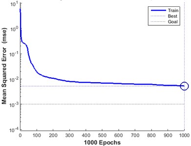
Table 3Result of bearing fault on outer ring
Sample | Expected output | Real output of BP neural network | Result | ||||||
1 | 0 | 1 | 0 | 0 | –0.0292 | 1.0255 | –0.0184 | 0.0218 | True |
2 | 0 | 1 | 0 | 0 | –0.0251 | 0.9344 | 0.0681 | 0.0222 | True |
3 | 0 | 1 | 0 | 0 | –0.0374 | 0.9244 | 0.0786 | 0.0340 | True |
4 | 0 | 1 | 0 | 0 | 0.0381 | 0.9062 | 0.0900 | –0.0347 | True |
5 | 0 | 1 | 0 | 0 | –0.0077 | 1.0168 | –0.0140 | 0.0047 | True |
Diagnostic accuracy | 100 % | ||||||||
Table 4The results of BP neural network diagnosis
Type | Normal | Outer ring fault | Inner ring fault | Rolling body fault |
Accuracy | 100 % | 100 % | 100 % | 80 % |
4. Conclusion
In this paper, an intelligent diagnosis system of train rolling bearings based on Sparse Fast Fourier Transform was proposed. It can be used to solve the problem that traditional diagnosis system based on FFT always leads to very high hardware cost when monitoring a large number of datum from all bearings in a train. Because most vibration signals in frequency domain are sparse, the SFFT algorithm can realize a faster way of performing Discrete Fourier Transforms with only a few nonzero Fourier coefficients of signals. The experimental results in Table 3 and 4 of Section 3.3 indicate the proposed method possesses the validity on the premise that the key signal is not lost. It is of great significance for diagnosing bearing fault on-line, locking location and fault type accurately.
References
-
Anna C. G., Yi L., Ely P., et al. Approximate sparse recovery: optimizing time and measurements. SIAM Journal on Computing, Vol. 41, Issue 2, 2012, p. 436-453.
-
Mark A. A Faster Fourier Transform. MIT Technology Review, 2012, http://www2.technologyreview.com/article/427676/a-faster-fourier-transform/.
-
Haitham H., Fadel A., Dina K., et al. Faster GPS via the sparse Fourier transform. Proceedings of the 18th Annual International Conference on Mobile Computing and Networking, 2012, p. 353-364.
-
Haitham H., Piotr I., Dina K., et al. Nearly Optimal Sparse Fourier Transform. Arxiv Preprint arXiv:1201.2501, Version 1, 2012, p. 28.
-
Haitham H., Piotr I., Dina K., et al. Simple and practical algorithm for sparse Fourier transform. Proceedings of the 23rd Annual ACMSIAM Symposium on Discrete Algorithms, 2012, p. 1183-1194.
-
Haitham H., Piotr I., Dina K., et al. Sparse Fast Fourier Transform Code Documentation. 2012.
-
Jörn S. High Performance Sparse Fast Fourier Transform. Department of Computer Science in ETH Zurich, 2013.
-
Xin Y. Research on Service Process Monitoring and Fault Diagnosis System of Train Bogie Bearing. Beijing Jiaotong University, 2012, (in Chinese).
-
Xiaofeng L., Limin J., Xin Y. Fault diagnosis of train axle box bearing based on multifeature parameters. Discrete Dynamics in Nature and Society, Vol. 2015, 2015, p. 846918.
-
Zhenzhen S. Application of Fourier transform and wavelet transform in signal de-noising. Journal of Electronic Design Engineering, Vol. 4, 2011, p. 155-157, (in Chinese).
-
Yiding H., Weixin R., Dong Y., et al. Demodulation of non-stationary amplitude modulated signal based on Hilbert transform. Journal of Vibration and Shock, Vol. 32, Issue 10, 2013, p. 181-183, (in Chinese).
-
Kwak J. S., Song J. B. Trouble diagnosis of the grinding process by using acoustic emission signals. International Journal of Machine Tools and Manufacture, Vol. 41, Issue 6, 2001, p. 899-913.
-
Kleinbaum D. G., Klein M. Introduction to Logistic Regression. Logistic Regression. Springer, New York, 2010, p. 1-39.
-
Zhou Z. H., Chen Z. Q. Hybrid decision tree. Knowledge-Based Systems, Vol. 15, Issue 8, 2002, p. 515-528.
-
Bishop C. M. Neural Networks for Pattern Recognition. Oxford University Press, 1995.
-
Benediktsson J., Swain P. H., Ersoy O. K. Neural network approaches versus statistical methods in classification of multisource remote sensing data. IEEE Transactions on Geoscience and Remote Sensing, Vol. 28, Issue 4, 1990, p. 540-552.
-
Kosbatwar S. P., Pathan S. K. Pattern association for character recognition by back-propagation algorithm using neural network approach. International Journal of Computer Science and Engineering Survey, Vol. 3, Issue 1, 2012, p. 127-134.
-
McClelland J. L., Rumelhart D. E. Parallel Distributed Processing: Explorations in the Microstructure of Cognition. Vol. 1, MIT Press, 1986, p. 547.
-
Verma A. K., Cheadle B. A., Routray A., et al. Porosity and permeability estimation using neural network approach from well log data. GeoConvention Vision Conference, Canada, 2012.
About this article

This paper is supported by the National High-Tech Research and Development Program of China (Grant No. 2011AA110503).
