A novel manifold learning denoising method on bearing vibration signals

Gao, Jingwei; Wang, Ruichen; Hu, Lei; Zhang, Rui

Journal of Vibroengineering

Browse Journal

Submit article

Published: 15 February 2016

Check for updates

A novel manifold learning denoising method on bearing vibration signals

Jingwei Gao¹

Ruichen Wang²

Lei Hu³

Rui Zhang⁴

^{1, 3, 4}National University of Defense Technology, Changsha, China

²University of Huddersfield, Huddersfield, UK

Corresponding Author:

Jingwei Gao

Cite the article Download PDF

Downloads 1279

Abstract

Bearing failures are a major source of problem in rotating machines. These faults appear as impulses at periodic intervals resulting in form of specific characteristic frequencies. However, the characteristic frequencies are submerged in noise causing by a result of small imperfections in the balance or smoothness of the components of the bearing. To retrieve the characteristic fault frequencies of the vibration signal, signal denoising is an essential processing step in fault diagnosis of the bearings. This paper presents time-frequency analysis and nonlinear manifold learning technique for denoising vibration signals corrupted by additive white Gaussian noise. According to keeping the computing time acceptable, a novel manifold learning denoising method is put forward combining data compression and reconstruct operations. Simulation and experiments are employed to verify the feasibility and effectiveness of the proposed method on bearing vibration signals. Furthermore, this method can be used in other fault detection fields, such as engine, suspension device, and vehicle structures.

1. Introduction

Bearing failure, one of the most common causes of faults in rotating machines, can be catastrophic and result in costly downtime [1]. Abrasion, fatigue, and pressure-induced welding are three primary causes of bearing failure. Although these three causes are known, an operator cannot predict when the failure will occur. Thus, early fault detection in rotating machineries is useful in terms of system maintenance and process automation, which will help to save millions on emergency maintenance and production costs [2].

Vibration analysis is a very powerful condition monitoring technique which is becoming more popular and common practice in industry, for its effectiveness and easy manipulation [3]. When bearing defects take place, the vibration signals tend to show unstable, nonlinear behaviors due to variable load, stiffness, uneven clearance and background random noise. Under a high-level signal noise ratio(SNR), vibration feature caused with faulty component of bearing would be extracted from vibration signals using appropriate data analysis algorithms, such as Envelope Analysis [4], Time-Frequency Analysis (TFA) [5], Wavelet Analysis (WA) [6], Empirical Mode Decomposition (EMD) [7], Hilbert-Huang Transform (HHT) [8], Modulation Signal Bispectrum (MSB) [9], Quantum Theory (QT) [10], etc.

However, the challenge of monitoring the working condition of bearing based on vibration signal analysis is how to extract the fault feature accurately under a lower-level SNR and using acceptable calculation time. Therefore, the vibration signals denoising algorithm should composed of two key points, one is the algorithm could separate the periodic vibration signals from the original bearing signals which may contain lots of nonlinear behaviors and strength random noise. The other is the computing time may be acceptable, because an early fault would develop to a severe fault after a long-time calculation time.

In recent years, manifold learning (ML) was used in the fault diagnosis of rotating machines due to its advantages in nonlinear feature extraction [11, 12]. Manifold learning can identify a low-dimension nonlinear structure hidden in high-dimension data through several analysis methods, including isometric feature mapping (IsoMap) [13], Locally Linear Embedding (LLE) [14], Laplacian Eigenmaps [15], Semidefinite Embedding [16], and local tangent space alignment (LTSA) [17], etc. The LTSA algorithm has been choose to denoising bearing vibration signals, and the effectiveness has been preliminary proved on several experiments [18-20].

But, we also notice that the calculation amounts of manifold learning method are huge which would cause unacceptable time in practice. One possible solution to the above problem is to reduce the amount of input data of the manifold learning method. In this paper, the time-frequency analysis results of the vibration signals was compressed to a lower dimension data using resampling algorithm as the inputs of the manifold learning method, while the outputs of the manifold learning method were executed data interpolation operation to reconstruction to a same size of the original data. Therefore, an improved manifold learning denoising method based on the above approach was put forward. By means of simulation and experiment studies on bearing fault detection, the effectiveness of the improved manifold learning method is verified and the calculation time is acceptable.

2. Improved manifold learning denoising method

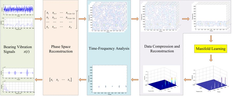
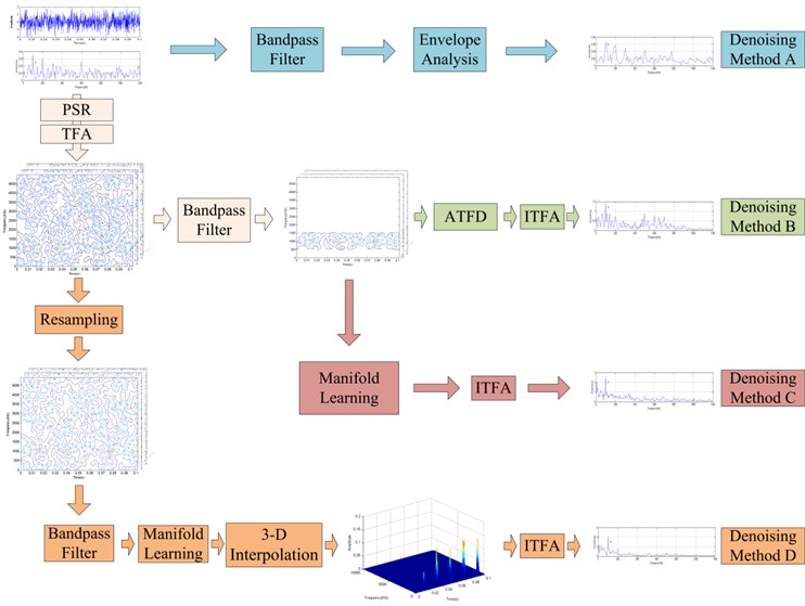
According to nonlinear behaviors of the bearing vibration signals and huge calculation during time-frequency analysis, an improved manifold learning denoising method (IMLDM) using PSR, TFA, ML and Date Compression and Reconstruction (DCR) is put forward and the flow diagram of IMLDM is given in Fig. 1.

Fig. 1The flow diagram of the improved manifold learning denoising method

2.1. Phase space reconstruction

PSR is an effective method to reconstruct an inherent dynamic system that is embedded in an observed time series, which aims to trace out the orbit of the dynamic system in the reconstructed high-dimension space [21]. Embedding dimension m and time delay factor $τ$ are the key two influence factors of PSR. For a given $N$ points time series, the m-dimension phase space is given as:

1

X_{N} (m, τ) = [\begin{array}{l} x_{1} & x_{1 + τ} & \dots & x_{1 + (m - 1) τ} \\ x_{2} & x_{2 + τ} & \dots & x_{2 + (m - 1) τ} \\ \dots & \dots & \dots & \dots \\ x_{n} & x_{n + τ} & \dots & x_{N} \end{array}],

where $x_{i}$ is the $i$ th data point in the given time series $x (t)$ , $τ$ is time delay and $n = N - m + 1$ . The precision of $m$ and $τ$ is directly related with the accuracy of the invariables of the described characteristics of the strange attractors in PSR. But when the embedding dimension $m$ increasing and the time delay $τ$ decreasing, the phase space matrix $X_{N} (m, τ)$ will be enlarged rapidly and will need huge calculation in the following analysis. Then it is very important to select a suitable pair of embedding dimension $m$ and time delay $τ$ when performing the PSR.

According to [22], embedding dimension $m$ and time delay $τ$ are closely related because the time series in the real world could not be infinitely long and could hardly avoid being noised. In this paper, the time window $t_{w} = (m - 1) τ$ is selected for the reconstruction of the phase space.

2.2. Time-frequency analysis

TFA is a body of techniques and methods used for characterizing and manipulating signals which is proved its advantages in vibration signal processing. In this paper, the short-time Fourier transform (STFT) is selected, and it is obtained by taking the discrete-time Fourier transform (DTFT) of each windowed block $u$ :

2

S (u, w) = D T F T \{x (n) w (n - u \frac{N}{2})\} .

The inverse STFT begins with the inverse DTFT of $S (u, w)$ to recover $s (u, n)$ :

3

s (u, n) = D T F T^{- 1} \{S (u, w)\},

where the window function is the $N$ -point half-cycle sine window, $ω (n) = s i n (π (n + 0.5) / N)$ , $n = 0,…, N - 1$ .

2.3. Data compression and reconstruction

In order to decrease the calculation, data compression and reconstruction is applied after STFT and before ISTFT. According to keeping the orient characteristics of the original vibration signals using less amount of data, data resampling, image bandpass filtering, 3-D interpolation are used in the paper.

For a given $N$ points signals, a time-frequency distribution matrix with the size of $N$ × $N$ could be obtained using the Eq. (2). Using data resampling algorithm, all time-frequency distribution matrix were re-sampled to be ( $N / N_{c}$ )×( $N / N_{c}$ ) matrices, where $N_{c}$ is the resampling coefficient.

The time-frequency distribution (TFD) matrix can be classified to two frequency band parts. One is the frequency band of energy concentration area containing most orient information. The other is the rest frequency bands which random noise is the main component rather than periodic signals. Therefore, only the frequency band of energy concentration area is useful for the time-frequency analysis. According to the maximum value of the time-frequency distribution matrix are usually occurs in the frequency band of energy concentration area, a frequency band $B (f, f_{b})$ containing the maximum value of the time-frequency distribution matrix is defined as:

4

B (f, f_{b}) = [\begin{array}{l} f - f \times f_{b} & f + f \times f_{b} \end{array}],

where $f$ is the frequency value where the maximum value of the time-frequency distribution matrix is obtained, and $f_{b}$ is the filter coefficient. Thus, an image bandpass filtering will be applied in the TFD using the given frequency band.

Data resampling can compressing the dimension of the analyzed TFD matrix, but also can lead to signal distortion when executing ISTFT due to low dimension of the TFD matrix. A 3-D interpolation method is used to recover the TFD data from the resampling data using the interpolation coefficient $I_{c}$ is the reciprocal value of $N_{c}$ .

2.4. Manifold learning

Many high-dimension data sets of dynamic system can be modeled as sets of points or vectors lying close to a low-dimensional nonlinear manifold. Manifold learning aims at discovering the intrinsic structure of the time-frequency distribution matrix. In this step, the LTSA algorithm is employed to extract the intrinsic manifold from $m$ time-frequency distribution matrix and two new time-frequency distribution matrix can be obtained. One time-frequency distribution matrix contains the most periodic information of the vibration signals, while the other one reflects the random noise of the vibration signals. The details of the LTSA is given in [17].

In summary, the procedure of the improved manifold learning denoising method for bearing vibration signals processing can be described in the following steps:

(1) Sampling a vibration signal with $N$ points data, and use PSR to construct a $m$ × $n$ data matrix $X_{N} (m, τ)$ .

(2) Use TFA to get the STFT spectrum for each row of the matrix $X_{N} (m, τ)$ .

(3) Obtain a set of low dimension matrix by resampling the matrix $X_{N} (m, τ)$ , and extract image bandpass filtering through a frequency band $B (f, f_{c})$ .

(4) Transform the 3-D matrix to a 2-D matrix to satisfy the input of LTSA by transform each 2-D time-frequency distribution matrix to a 1-D vector, and use LTSA algorithm to train the TFD matrix.

(5) Use a 3-D interpolation method to recover the TFD data from the resampling data.

(6) A new time series with $N$ points will be generated by ISTFT.

3. Simulation verification

3.1. Simulation signal

A simulation example is given to demonstrate the improved manifold learning denoising method for bearing vibration signals processing. The simulated signal is constructed by considering a single degrees of freedom vibration system with damping as follows:

5

x (t) = \sum_{i = 1}^{s} A e x p \{\frac{- ς}{\sqrt{1 - ς^{2}}} [2 π f_{0} (t - i d)]^{2}\} s i n [2 π f_{0} (t - i d)] + n (t),

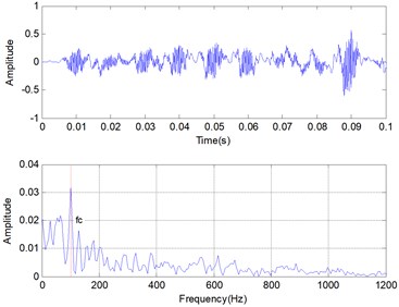
where the basic frequency $f_{0} =$ 3000 Hz, the impulse period $d =$ 0.01 s, the damping ratio $ς =$ 0.01, the varying initial amplitude $A$ is set to 1, and $n (t)$ is the Gaussian noise. The sampling frequency $f_{s} =$ 12000 Hz, the total amount of sampling points $N =$ 2048 $+ m - 1$ and the signal-to-noise ratio (SNR) is set to near –10 dB. The time domain and frequency domain of the simulation vibration signals with noise are given respectively in Fig. 2.

Fig. 2Time domain and frequency domain of simulation vibration signal

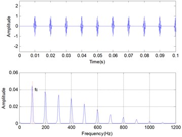
a) Simulation signal without noise

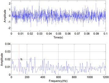
b) Simulation signal with predicted noise

From the frequency domain of simulation signals using fast Fourier transform (FFT), the characteristics frequency $f_{c} =$ 100 Hz is submerged in noise.

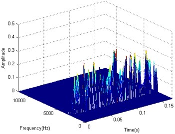
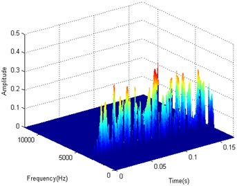
In the step of PSR, the time window $t_{w} = (m - 1) τ$ ( $m =$ 20, $τ =$ 1) is selected, and a 20×2048 data matrix $X_{N} (m, τ)$ is construct using 2067 points. Due to the length of each signals is equal to 2048, $m$ TFD matrix with the size 2048×2048 are generated using STFT. One of the TFD matrix is given in Fig. 3(a). Using the calculation steps in Section 2.2, the resampling coefficient $N_{c}$ is set to 8, and $m$ TFD matrix with the size 256×256 are obtained, which one of the resampling TFD matrix is shown in Fig. 3(b). Comparing with the two figures in Fig. 3, it can be seen that the resampling matrix can keep the original features of the TFD matrix, while the size of each TFD matrix is changed from 2048×2048 to 256×256.

Fig. 3Time-frequency distribution matrix of simulation vibration signal

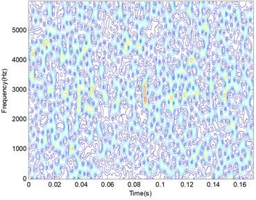
a) Time-frequency distribution 2048×2048

a) Time-frequency distribution 256×256

After resampling the TFD matrix, the maximum value of the TFD matrix will be calculated in order to determine the filter band of the TFD matrix. In this simulation signals, the maximum value of the TFD matrix is occurring near the basic frequency $f_{0}$ , which means the highest energy contributions are located in the frequency band near basic frequency $f_{0} =$ 3000 Hz. The filter coefficient $f_{b}$ is set to 0.1, and the filter band will be determined from 2700 Hz to 3300 Hz. The TFD matrix using bandpass filtering is give in Fig. 4(a).

Fig. 4Manifold learning results of simulation vibration signal

a) Original TFD 256×256

b) Periodic manifold 256×256

c) Random manifold 256×256

d) Manifold learning result 256×256

When using the LTSA algorithm to train the $m$ TFD matrix, several parameters are need to determined. In this paper, the target dimension is set to 3, while the nearest neighbors are set to 8. After training by the LTSA algorithm, three TFD matrix will be obtained, which the first one represents the periodic manifold of the signal while the rest two matrix represents the random manifold of the signal. The periodic manifold of the signal is shown in Fig. 4(b). Comparison Fig. 4(b) to Fig. 4(a), we can see that the main periodic information of the vibration signal was reserved perfectly. One of the random manifolds of the signal is shown in Fig. 4(c), which is represent noise of the signals. When the periodic manifold of the signal is selected instead of the original TFD, the random manifold of the signal will be removed from the original signal. Then the final manifold learning result is obtained though a simple threshold filter on the periodic manifold of the signal, which is shown in Fig. 4(d).

Due to the data compression of the TFD matrix, the manifold leaning result are a matrix with the size of 256×256, which is shown in Fig. 5(a). In order to recover the initial information of the vibration signal, a 3-D interpolation method will be applied. The interpolation coefficient $I_{c}$ is set to 0.125 for the resampling coefficient $N_{c}$ is set to 8. The interpolated TFD matrix with the size of 2048×2048 is given in Fig. 5(b).

Fig. 53-D interpolation result of TFD matrix

a)

b)

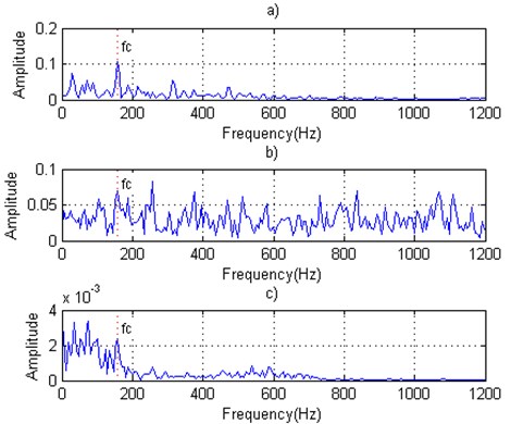
The denoising vibration signal will be generated using ISTFT on the interpolated TFD matrix. Denoising result of simulation signal in time domain and frequency domain are shown in Fig. 6. From the figure, we can see the periodic impulse in time domain and the characteristic frequency in frequency domain clearly.

Fig. 6Denoising result of simulation signal in time domain and frequency domain

3.2. Comparison with other denoising methods

As a comparison, other traditional denoising methods have been also applied to extract the defective features from the vibration signal with noise. These methods include envelope analysis denoising method, time-frequency analysis bandpass filtering method, manifold learning without DCR method, and the proposed manifold learning denoising method with DCR, which is recorded as denoising method A-D. Fig. 7 gives the processing sequence of four denoising methods, and the similar and difference steps among the four denoising methods are given.

Fig. 7The processing sequence of four denoising methods

The above four denoising methods are applied for the simulation signals with different SNRs, and the denoising result for the simulation signal with SNR $=$ –10 dB is given in Fig. 8.

To evaluate the result of the proposed method quantitatively, a new parameter, the energy distribution percent of characteristic frequencies (CF) is put forward. The CF use the total amplitude of characteristic frequencies divided by the total amplitude of the whole frequencies in frequency domain. The CFs of four denoising methods for different SNRs is shown in Fig. 9.

From the Fig. 9, it can be seen that the four denoising method can denoise the simulation signal very well, when the SNR of the signal is –5 dB. The denoising method A will be useless when the SNR change to –10 dB, while the other methods are all effectively. When the SNR increasing to –15 dB, it is difficult for the denoising method B to denoising the vibration signal with strength noise. The denoising method C and D can also obtain better denoising results due to their ability on nonlinear denoising between –15 dB and –16.5 dB. Four denoising methods will be all ineffective when the SNR reach –18 dB.

Table 1Computing time of four denoising methods for different SNR (s)

Denoising method	SNR (dB)
Denoising method	–5	–10	–15	–16.5	–18	–20
A	0.0275	0.0189	0.0160	0.0195	0.0192	0.0221
B	54.6228	53.6784	58.4070	53.7034	59.3431	56.0113
C	8235.0225	8143.3075	8337.6147	8634.3248	8499.2228	8552.1589
D	136.1097	114.1047	138.8496	135.4027	200.3265	153.9839

Computing time is another key parameter in comparison with four denoising methods. Computing time of four denoising methods for different SNRs using the computer Surpace Pro 3 with I5 CPU and 4 G memories is given in Table 1. From the Table 1, it can be seen that computing time for method A, B and D is acceptable, while the time for method C are much longer than the other three methods.

Fig. 8Denoising result of four denoising methods for the simulation signal with SNR = –10 dB: a) Simulation signal without noise, b) Simulation signal with noise, c) Denoising signal using denoising method A, d) Denoising signal using denoising method B, e) Denoising signal using denoising method C, f) Denoising signal using denoising method D

Denoising result of four denoising methods for the simulation signal with SNR = –10 dB: a) Simulation signal without noise, b) Simulation signal with noise, c) Denoising signal using denoising method A, d) Denoising signal using denoising method B, e) Denoising signal using denoising method C, f) Denoising signal using denoising method D

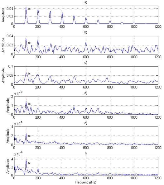
Fig. 9The CFs of four denoising methods for different SNRs

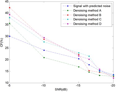
Combing the denoising results and computing time, the proposed denoising method is demonstrated to be feasibility and effectiveness for simulation vibration signals with the SNR is bigger than –16.5 dB.

4. Experimental verification

In order to verify the effectiveness of the new manifold learning denoising method for bearing vibration signals processing, a set of vibration signals provided by the Bearing Data Center of Case Western Reserve University(CWRU) were used. The bearing experiment system is shown in Fig. 10.

Fig. 10Bearing experiment system

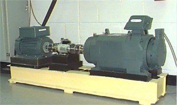
The bearing experiment system consists of a test bearing, a motor, a torque sensor, a dynamometer, and control system. A 2-hp, three-phase induction motor was connected to a dynamometer and torque sensor via a self-aligning coupling. The dynamometer was controlled to achieve expected torque load levels. The ball bearings were SKF 6205 with deep grooves. Single point faults were set on the test bearings at inner race, outer race and roller element through electro-discharge machining. Accelerometers were used for vibration data collection at a sampling frequency of 12 kHz, which were adhered to the housing with magnetic bases. The parameters of the three types of bearing defects are listed in Table 2.

In this section, an experiment is implemented to verify its feasibility and effectiveness in bearing vibration signals processing and its flow diagram is given in Fig. 11.

Fig. 11The flow diagram of the experiment verification method

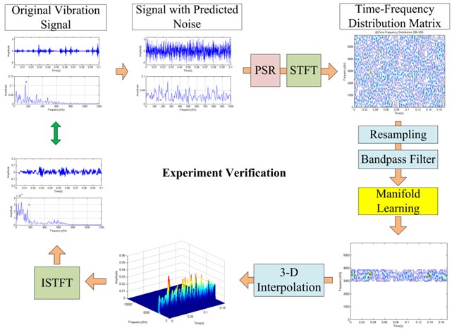
Due to CWRU data are collected in laboratory conditions and in order to test the performance of the proposed denoising method in real world industrial situation, three bearing defect vibration signals were generated with additional predicted noise, which the relative SNR is about –10 dB. When using the proposed denoising method, the parameters are selected as shown in Table 3.

Table 2Parameters of the bearing defects

Bearing defect type	Defect depth (in)	Defect width (in)	Motor load (hp)	Motor speed (rpm)	$f_{c}$ (hz)
Inner race defect	0.011	0.014	0	1797	158.1
Outer race defect	0.011	0.014	0	1748	104.5
Roller element defect	0.011	0.014	0	1749	141.0

Table 3Sampling parameters of the bearing defect vibration signals

Bearing defect type	$N$	Snr	$M$	$τ$	$N_{c}$	$f_{0}$	$I_{c}$
Inner race defect	2048	–12.14	20	1	8	0.1	0.125
Outer race defect	2048	–11.53	20	1	8	0.15	0.125
Roller element defect	4096	–9.56	20	1	16	0.1	0.0625

4.1. Bearing vibration signal denoising with inner race defect

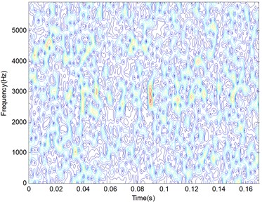
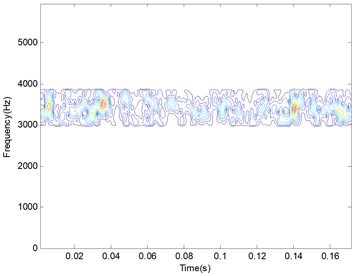
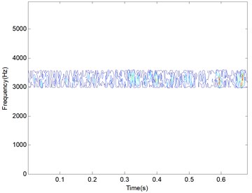
The bearing vibration signal with inner race defect are analyzed using the above experiment verification method given in Fig. 11. After executing PSR on the original signals, a new matrix with the size of 20×2048 will be obtained. Then 20 TFD matrix will be calculated using each column of the above matrix. An original TFD of the inner race defect is shown in Fig. 12(a) and the resampling result of the TFD is given in Fig. 12(b).

Fig. 12An original TFD and resampling TFD of inner race defective bearing signal

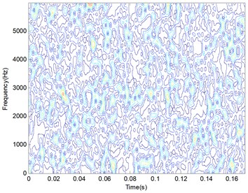
a) Time-frequency distribution 2048×2048

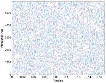
a) Time-frequency distribution 256×256

As we know, the TFD can indicate a combination of time domain information and frequency domain information. When the SNR of the signal is high, there are a series of impulse vibration in the time domain for the periodic contact of the bearing elements, which will cause periodic peaks appearing in a specific frequency band clearly. And due to the corruption of a high energy noise, the periodic information will be immerged in the time-frequency domain. From the Fig. 12(a), it can be seen that there are a series of peaks appearing near the 2900 Hz line and several peaks occurring randomly in the whole time-frequency domain.

Compared with the two TFDs in Fig. 12, the main distribution information of the time-frequency domain is kept in the resampling TFD instead of the original TFD. And the matrix size is decreased from 2048×2048 to 256×256 when the resampling coefficient is set to 8.

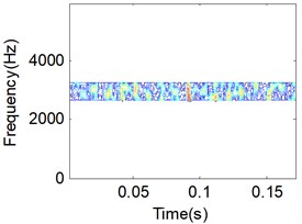
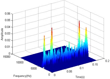
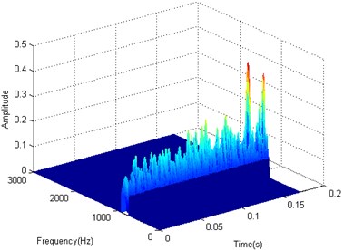
The manifold learning LTSA method is applied to the filtered signals using the frequency band between 2600 Hz to 3200 Hz. The target dimension is set to 3, while the nearest neighbors are set to 8. The first TFD matrix is selected as the training result of manifold learning, and its 2-D and 3-D distribution figures are given in Fig. 13(a) and (b).

Fig. 13Manifold learning result of inner race defective bearing signal

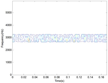
a) 2-D distribution figure

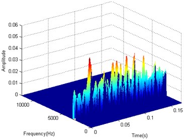
b) 3-D distribution figure

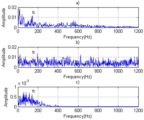
By the inverse TFA operation, the frequency spectrum of the signal is shown in Fig. 14(c). Comparing with the original signal sampling on the test rig and the signal with predicted noise which is shown in Fig. 14(a) and (b), the characteristic frequency is appeared clearly in the frequency spectrum of the denoising signal, while the characteristic frequency is submerged in the frequency domain of signals with predicted noise. The result proves that the proposed manifold learning denoising method can reduce noise effectively and keep the instinct information of the original signal.

4.2. Bearing vibration signal denoising with outer race defect

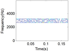
Similarity, the way of denoising method for inner race defect is applied for outer race defect. Due to the difference of the rotating speed and the characteristics frequency, the filter band is selected from 3000 Hz to 3900 Hz. The other parameters are the same. The manifold learning result of bearing vibration signal is given in Fig. 15.

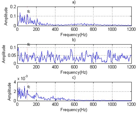
Fig. 14Inner race defective bearing signals: a) Inner fault original signal, b) Inner fault signal with predicted noise, c) Inner fault denoising signal

Inner race defective bearing signals: a) Inner fault original signal, b) Inner fault signal with predicted noise, c) Inner fault denoising signal

Original signal, signal with predicted noise and denoising signal of the bearing outer race defect are shown in Fig. 16.

The fault characteristic frequency $f_{c} =$ 104.5 Hz can be reproduced in the frequency spectrum of the signal after denoising the signal using the manifold learning method.

Fig. 15Manifold learning result of outer race defective bearing signal

a) 2-D distribution figure

b) 3-D distribution figure

Fig. 16Outer race defective bearing signals: a) Outer fault original signal, b) Outer fault signal with predicted noise, c) Outer fault denoising signal

Outer race defective bearing signals: a) Outer fault original signal, b) Outer fault signal with predicted noise, c) Outer fault denoising signal

4.3. Bearing vibration signal denoising with roller element defect

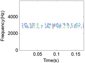
The roller element defective bearing vibration signal is analyzed to verify the proposed denoising method. The frequency spectrum of roller element defective bearing vibration signal is more complex than the signals of inner/outer race defect. There are several other frequency components existing close to the characteristic frequency $f_{c}$ . Then in order to separate the useful frequency information from the other frequency information, more sampling points are chosen and a large PSR matrix is generated which will increase the calculation amounts. A higher resampling coefficient $N_{c} =$ 16 and a lower interruption coefficient $I_{c} =$ 0.0625 are selected for saving the computing time.

The manifold learning result and the denoising signal of the roller element defective bearing vibration signal are given in Fig. 17 and Fig. 18. From the Fig. 18, the characteristic frequency can also be found from the frequency spectrum of the denoising vibration signal. However, in compared with the denoising result for inner/outer race defect, the lower frequency components will be enhanced and will cause decreasing the detection accuracy in the following bearings fault diagnosis.

In order to verify the computing time is acceptable, the computing time for each detective signal is recorded and is shown in Table 4. The average computing time is about 150 s using the same computer in Section 3, which can be used on the online condition monitoring for bearings.

Table 4Computing time for bearing vibration signals

Bearing defect type	Inner race defect	Outer race defect	Roller element defect
Computing time (s)	136.76	138.02	186.23

Fig. 17Manifold learning result of roller element defective bearing signal

a) 2-D distribution figure

b) 3-D distribution figure

Fig. 18Roller element defective bearing signals: a) Roller fault original signal, b) Roller fault signal with predicted noise, c) Roller fault denoising signal

Roller element defective bearing signals: a) Roller fault original signal, b) Roller fault signal with predicted noise, c) Roller fault denoising signal

5. Conclusions

A novel manifold learning denoising method was put forward in this paper and the effectiveness of the new denoising method is verified by means of numerical simulation and experiment studies on bearing fault detection. Based on the analysis results, we can draw the following conclusions:

1) The manifold learning denoising method can keep the intrinsic periodic information from the vibration signals with additional predicted noise, and the computing time is acceptable due to apply data compression and reconstruction in improving the manifold learning denoising method.

2) The performance of the proposed denoising method has been proved better than the conditional denoising methods using numerical simulation.

3) The denoising method will enhance the lower frequency components and cause a weaker denoising result. The optimization of the manifold learning algorithm and the selected parameters need to perform in the future research.

References

Jiang F., Zhu Z., Li W., Chen G., Zhou G. Identification and diagnosis of concurrent faults in rotor-bearing system with WPT and zero space classifiers. Journal of Vibroengineering, Vol. 16, Issue 2, 2014, p. 901-912.

Search CrossRef
Kankar P. K., Sharma S. C., Harsha S. P. Fault diagnosis of ball bearings using machine learning methods. Expert Systems with Applications, Vol. 38, Issue 3, 2011, p. 1876-1886.

Search CrossRef
Zarei J., Tajeddini M. A., Karimi H. R. Vibration analysis for bearing fault detection and classification using an intelligent filter. Mechatronics, Vol. 24, Issue 2, 2014, p. 151-157.

Search CrossRef
Zhao F., Chen J., Guo L., Li X. Neuro-fuzzy based condition prediction of bearing health. Journal of Vibration and Control, Vol. 15, Issue 7, 2009, p. 1079-1091.

Search CrossRef
Feng Z., Liang M., Chu F. Recent advances in time–frequency analysis methods for machinery fault diagnosis: a review with application examples. Mechanical Systems and Signal Processing, Vol. 38, Issue 1, 2013, p. 165-205.

Search CrossRef
Bin G. F., Gao J. J., Li X. J., Dhillon B. S. Early fault diagnosis of rotating machinery based on wavelet packets – empirical mode decomposition feature extraction and neural network. Mechanical Systems and Signal Processing, Vol. 27, Issue 2, 2012, p. 696-711.

Search CrossRef
Lei Y., Lin J., He Z., Zuo M. J. A review on empirical mode decomposition in fault diagnosis of rotating machinery. Mechanical Systems and Signal Processing, Vol. 35, Issue 1, 2013, p. 108-126.

Search CrossRef
Pandya D. H., Upadhyay S. H., Harsha S. P. Fault diagnosis of rolling element bearing with intrinsic mode function of acoustic emission data using APF-KNN. Expert Systems with Applications, Vol. 40, Issue 10, 2013, p. 4137-4145.

Search CrossRef
Gu F., Wang T., Alwodai A., Tian X., Shao Y., Ball A. D. A new method of accurate broken rotor bar diagnosis based on modulation signal bispectrum analysis of motor current signals. Mechanical Systems and Signal Processing, Vol. 50, Issue 1, 2015, p. 400-413.

Search CrossRef
Chen Y., Zhang P., Wang Z., Yang W., Yang Y. Denoising algorithm for mechanical vibration signal using quantum Hadamard transformation. Measurement, Vol. 66, Issue 4, 2015, p. 168-175.

Search CrossRef
Tang B., Song T., Li F., Deng L. Fault diagnosis for a wind turbine transmission system based on manifold learning and Shannon wavelet support vector machine. Renewable Energy, Vol. 62, Issue 2, 2014, p. 1-9.

Search CrossRef
Raducanu B., Dornaika F. A supervised non-linear dimensionality reduction approach for manifold learning. Pattern Recognition, Vol. 45, Issue 6, 2012, p. 2432-2444.

Search CrossRef
Tsoli A., Jenkins O. C. Neighborhood denoising for learning high-dimensional grasping manifolds. IEEE/RSJ International Conference on Intelligent Robots and Systems, Nice, 2008, p. 3680-3685.

Search CrossRef
Roweis S. T., Saul L. K. Nonlinear dimensionality reduction by locally linear embedding. Science, Vol. 290, Issue 5500, 2000, p. 2323-2326.

Search CrossRef
Thorstensen N., Segonne F., Keriven R. Pre-Image as Karcher Mean using Diffusion Maps: Application to Shape and Image Denoising. Scale Space and Variational Methods in Computer Vision. Springer Berlin Heidelberg, 2009, p. 721-732.

Search CrossRef
McFee B., Lanckriet G. Partial order embedding with multiple kernels. ICML Proceedings of the 26th Annual International Conference on Machine Learning, New York, 2009, p. 721-728.

Search CrossRef
Zhang Z. Y., Zha H. Y. Principal manifolds and nonlinear dimensionality reduction via tangent space alignment. Journal of Shanghai University (English Edition), Vol. 8, Issue 4, 2004, p. 406-424.

Search CrossRef
Gan M., Wang C., Zhu C. A. Fault feature enhancement for rotating machinery based on quality factor analysis and manifold learning. Journal of Intelligent Manufacturing, 2015, p. 1-18.

Search CrossRef
He Q., Liu Y., Long Q., Wang J. Time-frequency manifold as a signature for machine health diagnosis. IEEE Transactions on Instrumentation and Measurement, Vol. 61, Issue 5, 2012, p. 1218-1230.

Search CrossRef
He Q., Wang X., Zhou Q. Vibration sensor data denoising using a time-frequency manifold for machinery fault diagnosis. Sensors, Vol. 14, Issue 1, 2013, p. 382-402.

Search CrossRef
Hennenfent G., Herrmann F. J. Seismic denoising with nonuniformly sampled curvelets. Computing in Science and Engineering, Vol. 8, Issue 3, 2006, p. 16-25.

Search CrossRef
Ma H. G., Han C. Z. Selection of embedding dimension and delay time in phase space reconstruction. Frontiers of Electrical and Electronic Engineering in China, Vol. 1, Issue 1, 2006, p. 111-114.

Search CrossRef

About this article

Received

25 September 2015

Accepted

13 December 2015

Published

15 February 2016

SUBJECTS

Fault diagnosis based on vibration signal analysis

Keywords

bearing

vibration signals denoising

manifold learning

time-frequency analysis

Acknowledgements

The work was supported by the National Natural Science Foundation of China (Grant No. 51575518 and 11402297). The authors would like to thank Case Western Reserve University of offering free download of the bearing data, and the anonymous reviewers for their valuable comments.

This is an open access article distributed under the Creative Commons Attribution License, which permits unrestricted use, distribution, and reproduction in any medium, provided the original work is properly cited.