Research on modeling and dynamic characteristics of complex coaxial rotor system

2.1. Finite element formulation

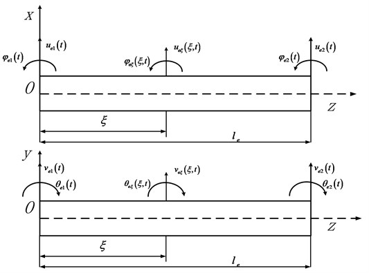
Fig. 1 shows the rotor element considered in this work. Each element consists of two nodes, with four degrees of freedom at each node, namely the lateral displacement and the slope. The lateral displacements in $X$ and $Y$ directions are denoted with $u$ and $v$ respectively. The slopes are denoted with $\theta$ and $\phi$ for angular displacements in $X$ and $Y$ directions respectively.

The nodal displacement vector can be described as:

The displacement vector within the element can be interpolated as:

The shape functions in Eq. (2) are:

Fig. 1Diagram of beam element

In Eq. (3), $l_e$ is the element length and $g$ is formulated as given below:

where $E_e$ the Young’s Modulus, $I_e$ the area moment of inertia, $G_e$ the shear modulus, $A_e$ the cross-sectional area. $\kappa$ is the shear coefficient, and for a hollow circular shaft section [16, 17]:

where $\mu$ is the Poisson’s ratio, $\lambda$ is the ratio of the inner shaft radius to the outer shaft radius. Hence for a solid shaft $\lambda \to 0$.

With rotary inertia and shear effects considered, the kinetic energy and strain energy for a shaft element is:

where ${\rho }_e$ denotes the density of the material and $\gamma$ is the transverse shear strain [18].

And thus the element mass matrix:

The element stiffness matrix:

where:

The element gyroscopic matrix:

where:

For disk element, the mass and gyroscopic matrices are:

where $m_d^i$, $I_d^i$ and $I_p^i$ are the mass, diametral moment of inertia and polar moment of inertia of the disk, respectively.

2.2. Nonlinear forces of the supports

For squeeze film dampers analyzed in this work, based on the short bearing assumption and the Reynolds boundary conditions, nonlinear forces of the SFD can be expressed as [19, 20]:

where $x$ and $y$ are the horizontal and vertical displacements of the journal. $I_j$ ($j=$1, 2, 3) are Sommerfeld integrals. $R$ and $L$ are radius and length of the SFD respectively. ${\mu }_s$ and $c$ denote the dynamic viscosity of the film and the radial clearance of the SFD.

As for the rolling ball bearing, based on pure rolling assumption and the Hertz contact theory, nonlinear force of the rolling ball bearing [21] is:

where the superscript $ir$ and $or$ in Eq.(14c) denote inner ring and outer ring of the bearing. $k_n$ in Eq.(14a) is the contact stiffness between rollers and rings. $N_b$ represent number of the rollers. $\xi =3/2$ for the rolling ball bearing used in the intermediate support. ${\theta }_j$ is the rotation angle of the$j$th roller at time $t$. $\gamma$ and ${\omega }_c$ are bearing radial clearance and rotational speed of the bearing retainer respectively. $u_{\theta j}$ is the elastic radial deformation of the $j$th roller. $r$and $R$ represent radius of the inner and outer ring. ${\omega }_{in}$ and ${\omega }_{out}$ are the rotational speeds of the inner and outer rings.

2.3. Equations of motion and numerical algorithm

Equation of motion of a nonlinear rotor system can be written as:

where ${\mathbf{F}}^{unb}$ is the unbalance force vector. ${\mathbf{F}}^{nonl}$ is the nonlinear forces exerted by the SFDs and rolling bearing in this work. $\mathbf{M}$, $\mathbf{K}$, and $\mathbf{G}$ can be obtained quite readily with elements formulated in Section 2.1.

Mathematically, the model is a set of nonlinear second order differential equations. The computational efficiency of which depends on the numerical methods applied and the total DOFs of the rotor system. To combine accuracy of the finite element model and computational efficiency, the fixed interface modal synthesis is applied to reduce dimension of the mathematical model and thus the computational effort.

Eq. (15) can be rewritten as:

where ${\mathbf{u}}_I$ can be interpreted as linear DOFs, with only unbalance forces acting on, while ${\mathbf{u}}_J$ represents the interface DOFs or nonlinear DOFs in this work, including all the nodes with nonlinear forces acting on.

According to fixed interface modal synthesis method, transformation between physical and modal coordinates is:

where ${\mathbf{\varphi }}_k$ – the mass normalized normal mode matrix, ${\mathbf{\varphi }}_c$ – the mass normalized constrained mode, $\mathbf{I}$ – unity matrix, ${\mathbf{q}}_k$ – the normal mode coordinates, $\mathbf{T}$ – the transformation matrix. ${\mathbf{\varphi }}_c$ is given as below:

In Eq. (16), let ${\mathbf{u}}_J=\mathbf{}$0 and neglecting the gyroscopic effects gives:

Solving the eigenvalue problem corresponding to Eq. (17c) gives the mass normalized normal mode matrix ${\mathbf{\varphi }}_k$ and the modal frequency ${\mathrm{\Omega }}_k$.

Substitute Eq. (17a) into Eq. (16) and premultiply with ${\mathbf{T}}^T$ to obtain the reduced equations of motion:

where:

where ${\mathrm{\Omega }}_r$ is the $r$th modal frequency obtained from Eq. (17c). ${\mathbf{F}}_I^{unb}$ is the unbalance force acting on linear DOFs. ${\mathbf{F}}_J^{nonl}$ is the nonlinear force acting on nonlinear DOFs.

And:

where ${\mathbf{F}}_J^{SFD}=\left[\begin{array}{ccc}{f}_{1x}^{sfd}& f_{1y}^{sfd}& \cdots \begin{array}{cc}{f}_{Nx}^{sfd}& f_{Ny}^{sfd}\end{array}\end{array}\right]$ is the nonlinear force vector exerted by SFDs which can be calculated with Eq. (13). ${\mathbf{F}}_J^B=\left[\begin{array}{ccc}{f}_x^b& f_y^b& -\begin{array}{cc}{f}_x^b& {-f}_y^b\end{array}\end{array}\right]$ is the nonlinear force vector exerted by rolling bearing which can be calculated with Eq. (14). ${\mathbf{k}}_{JJ}$ and ${\mathbf{c}}_{JJ}$ are given below:

where $k_{Ji}$ and $c_{Ji}$ are the stiffness and damping coefficients of the elastic support, respectively. $N$ is the number of elastic supports.

Rearranging Eq. (18) gives:

In Eq. (23), the vector ${\mathbf{q}}_k$ and ${\mathbf{u}}_J$ can be interpreted as linear and nonlinear DOFs of the reduced system respectively. Obviously, there is no nonlinear force acting on the linear DOFs. Thus, the explicit Newmark-$\beta$ method applies to Eq.(23a) while implicit Newmark-$\beta$ method applies to Eq. (23b).

According to assumptions of Newmark-$\beta$ method, in time interval $\left[\begin{array}{cc}{t}_n& t_{n+1}\end{array}\right]$:

where $t_{n+1}=t_n+\mathrm{\Delta }t$ and $\mathrm{\Delta }t$ is the time increment. The superscript $n$ and $n+1$ denote $t_n$ and $t_{n+1}$.

Following equations can be obtained from Eq. (24):

With:

Substituting Eq. (24)-Eq. (27) into Eq. (23) yields:

With:

Using Eq. (26) to substitute for ${\dot{\mathbf{u}}}_J^{\mathrm{n}+1}$ in Eq. (29g) and substitute the new Eq. (29g) into Eq. (28b) to yield nonlinear equations of ${\mathbf{u}}_J^{n+1}$. After solving Eq. (28b) for ${\mathbf{u}}_J^{n+1}$ with numerical algorithms, ${\mathbf{q}}_k^{n+1}$ can be obtained with ${\mathbf{u}}_J^{n+1}$ substituted into Eq. (28a). Thus ${\dot{\mathbf{u}}}_J^{n+1}$, ${\ddot{\mathbf{u}}}_J^{n+1}$, ${\dot{\mathbf{q}}}_k^{n+1}$, ${\ddot{\mathbf{q}}}_k^{n+1}$ and can be solved from Eq. (25) and Eq. (26). The process continues to repeat and move forward to find ${\mathbf{u}}_J^{n+2}$, and so on. When the iteration is over, the nonlinear response in physical coordinate system can be obtained from Eq. (17a).

Computational efficiency of solving Eq. (23) depends on solving Eq. (23b) while dimensions of Eq. (23b) depend on DOFs with nonlinear forces acting on. Thus, the computational efficiency can be greatly improved with the modeling technique and solving method described in this work.

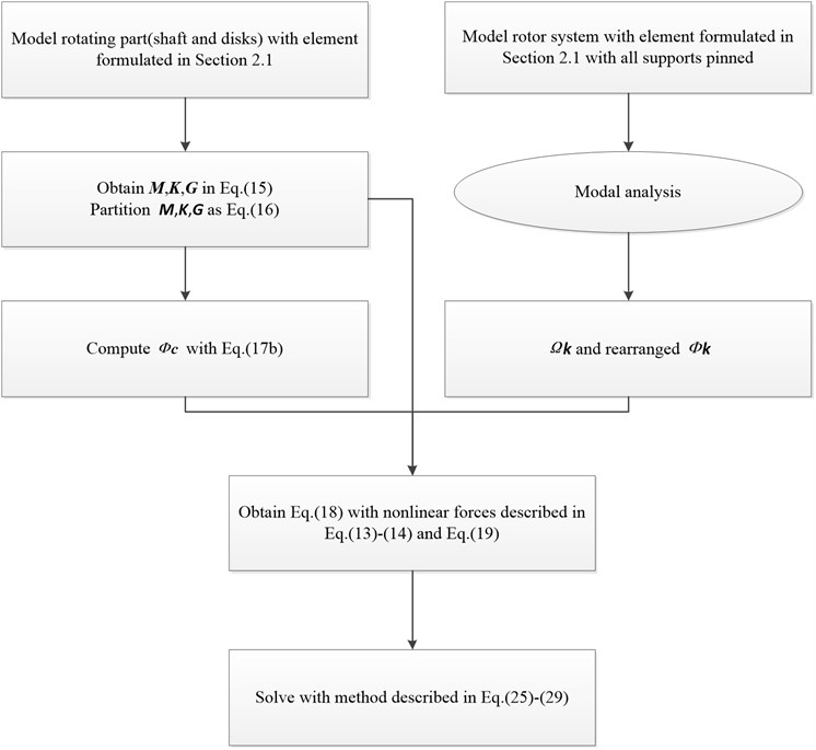
To summarize, nonlinear model of the rotor system is established with finite element method and fixed interface modal synthesis method; subsequently an implicit time-domain method based on Newmark-$\beta$ method is applied to solve the equations of motion of the reduced system thus dynamic characteristics can be obtained. The process of modeling and solving is described as follows: First, only the rotating components of the rotor assembly are modeled with the element described in Section 2.1 thus $\mathbf{M}$, $\mathbf{K}$ and $\mathbf{G}$ in Eq. (15) can be obtained and partitioned as Eq. (16) for calculating ${\mathbf{\varphi }}_c$ and later use. Then, in accordance with Eq. (17c), modal analysis is conducted on the model with all supports pinned to obtain ${\mathbf{\varphi }}_k$ and ${\mathrm{\Omega }}_k$. The left hand side of Eq. (18a) now is obtained with ${\mathbf{\varphi }}_k$, ${\mathbf{\varphi }}_c$ and the partitioned $\mathbf{M}$, $\mathbf{K}$ and $\mathbf{G}$ while the right hand side is formulated with Eq. (13), Eq. (14) and Eq. (19)-Eq. (22). Finally, Eq. (18a) is solved with the numerical method which is described by Eq. (23)-Eq. (29). Flowchart of the modeling and solving method is shown in Fig. 2.

Fig. 2Flowchart of modeling and solving

2.4. Test rig description

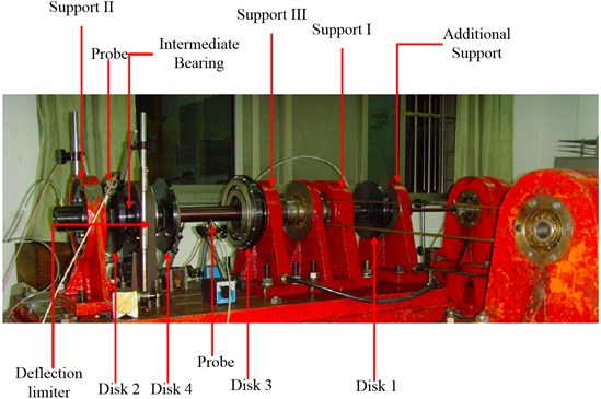
An overall view of the dual-rotor test rig is given in Fig. 3. The test rig was designed to study the dynamic characteristics of co-and counter-rotating dual-rotor systems with 4 or 5 supports. In this work, the 4 supports counter-rotating dual-rotor system is studied. So, the additional support in Fig. 3 was removed. Thus, the studied rotor system is designed with 4 supports and 4 disks, two for each rotor. The test rig consists of two shafts disposed along the same axis, connected by an intermediate bearing. Each shaft is driven by its own motor thus their spin speeds can be different. Speed ratio of outer and inner rotor is –1.65. Rear support of the outer rotor is intermediate support in which a rolling ball bearing is adopted. Support I and II are front and rear supports of inner rotor respectively while Support III and IV are front and rear support of outer rotor. The squirrel cage + rolling bearing + SFD supporting scheme is adopted for support I, II and III. While support IV, or the intermediate bearing, is mounted without SFD. Four eddy current probes are placed to measure the displacement of disk 2 and 4, two for each disk. It is to be noted that in Fig. 3 the eddy current probes have not been placed in the right positions yet.

The test profiles include slow run-up and run-down through the speed range of the test rig. The angular acceleration for inner rotor during run-up and rundown is approximately 10 rpm/s. Besides, the steady state response are measured when inner rotor spins at 128 rad/s, 160 rad/s and 210 rad/s. The operational ranges for the inner and outer rotor are 0-232 rad/s and 0-382 rad/s respectively. The excitation is only due to the residual unbalance of the rotors.

Fig. 3Dual-rotor test rig

3.1. Model introduction

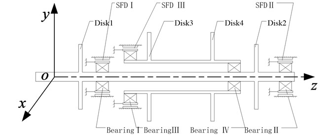
The counter-rotating coaxial system studied in this paper is presented in Fig. 4.

The stationary coordinate system in Fig. 4 consists of three mutually perpendicular axes, $ox$, $oy$, $oz$, intersecting at the point $o$ and axis of the rotor coincides with axis $oz$. The axes $ox$, $oz$ are horizontal, $oy$ is vertical.

Fig. 4Structural diagram of the coaxial rotor system

Model parameters of the rotor system studied in this work are listed in Table 1-5. The Young’s modulus of the shaft is 196 GPa, mass density 7810 kg/m³, and shear modulus 75.5 GPa. To apply modal synthesis method, 40 modes are retained in the normal mode matrix ${\mathbf{\varphi }}_k$. For the Newmark-$\beta$ method, $\alpha =$ 0.25, $\beta =$ 0.5.

Geometric dimensions and information of each element are listed in Table 1. Stiffness coefficients of elastic supports are listed in Table 2. Parameters of the intermediate bearing and SFDs are listed in Table 3 and 4. The unbalance configuration and inertia properties of each disk are listed in Table 5.

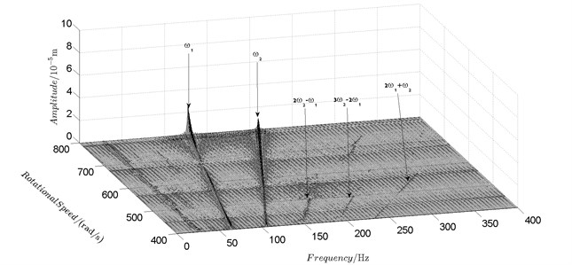
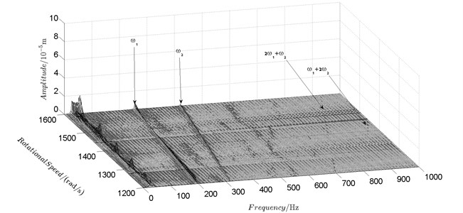
Fig. 5Spectrum cascade of the horizontal response of disk 2 and 4-numerical simulation

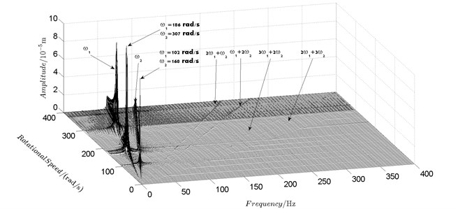
a) Disk 2

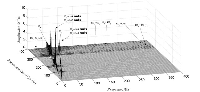
b) Disk 4

3.2. Unbalance response analysis

With the model established by method described in Section 2, steady-state unbalance response of the rotor system is obtained for rotational speed of the inner rotor varying from 4 rad/s to 1600 rad/s with a step length of 2 rad/s. Zero initial condition is adopted for the first step. For the rest steps, result of previous step is adopted as initial condition. Without loss of generality, unbalance response of disk 2 and disk 4 are analyzed to evaluate the coupling effect of the intermediate bearing.

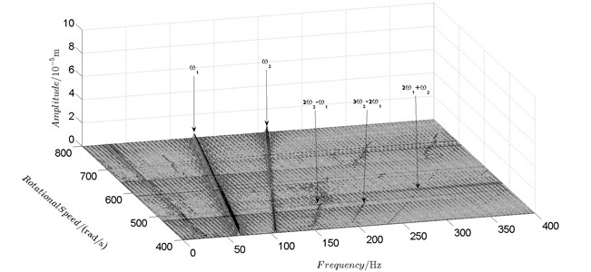
Fig. 6Spectrum cascade of the horizontal response of disk 2 and 4-experimental results

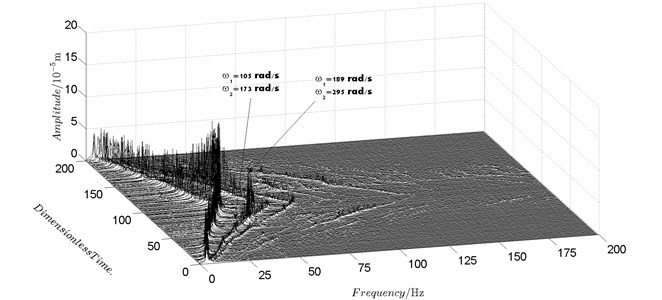
a) Disk 2

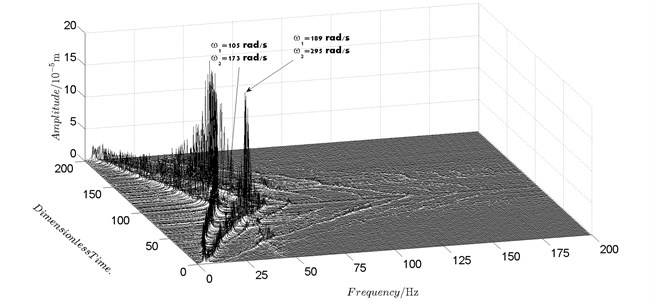
b) Disk 4

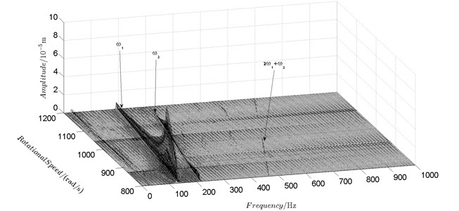
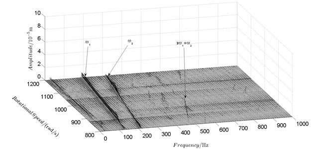
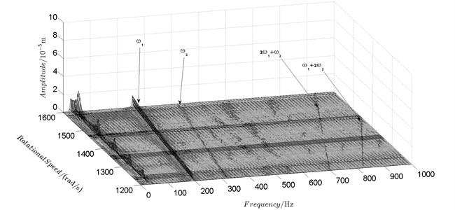
Spectrum cascades of the horizontal response of disk 2 and disk 4 with inner rotor operating in 4-400 rad/s are shown in Fig. 5 and Fig. 6. The simulation and experimental results are shown in Fig. 5 and Fig. 6 respectively. The numerically simulated spectrum cascades of the horizontal response of disk 2 and disk 4 with inner rotor operating in 400-1600 rad/s are shown in Figs. 7-9. Due to nonlinearities of SFD and the intermediate bearing as well as the multifrequency unbalance excitation of the inner and outer rotor, rich frequency components are observed in the response of disk 2 and disk 4. Following conclusions can be reached from Fig. 5-9:

(1) Responses of the inner and outer rotor are coupled because of the intermediate bearing. Frequency components, ${\omega }_1$ and ${\omega }_2$, corresponding to the unbalance excitation frequencies of the inner and outer rotor are dominant in the response of disk 2 and disk 4. The coupling effect also makes the spectrum cascades corresponding to disk 2 and disk 4 basically follow the same pattern with only slight differences in amplitude.

(2) Frequency components besides ${\omega }_1$ and ${\omega }_2$ in the responses of disk 2 and 4, such as ${2\omega }_1+{\omega }_2$, ${\omega }_1+{2\omega }_2$, ${3\omega }_1+2{\omega }_2$, ${2\omega }_1+3{\omega }_2$, $({\omega }_2-{\omega }_1)/2$, seen in Figs. 5-9, are mainly caused by the nonlinear forces of the SFD and the coupling effect of the intermediate bearing.

(3) By comparison between Fig. 5 and Fig. 7 it can be seen that the new combination frequency components, ${2\omega }_2-{\omega }_1\text{,}$${3\omega }_2-2{\omega }_1$emerge when inner rotor operating in 400-800 rad/s. However, ${2\omega }_2-{\omega }_1$ and ${3\omega }_2-2{\omega }_1$ are not observed for both disk 2 and 4 in Fig. 8 and Fig. 9 when the inner rotor operating in 800-1200 rad/s and 1200-1600 rad/s. Besides, ${2\omega }_1+{\omega }_2$ is persistent in 0-1600 rad/s for disk 2 and 4, which can be seen from Fig. 5 and Figs. 7-9.

(4) Two critical speeds of the rotor system, 168 rad/s and 186 rad/s, are observed in rotational speed range 0-200 rad/s in Fig. 5. The first one, 168 rad/s, is excited by the outer rotor and the second one, 186 rad/s, is excited by the inner rotor. It can be obtained from the experimental data shown in Fig. 6 that the corresponding critical speeds of the rotor system are 173 rad/s and 189 rad/s. Discrepancies of critical speeds between numerical and experimental results are less than 3 %, which demonstrate the validity of the model established in this work.

Fig. 7Spectrum cascade of the horizontal response of disk 2 and 4-numerical simulation

a) Disk 2

b) Disk 4

Fig. 8Spectrum cascade of the horizontal response of disk 2 and 4-numerical simulation

a) Disk 2

b) Disk 4

Fig. 9Spectrum cascade of the horizontal response of disk 2 and 4-numerical simulation

a) Disk 2

b) Disk 4

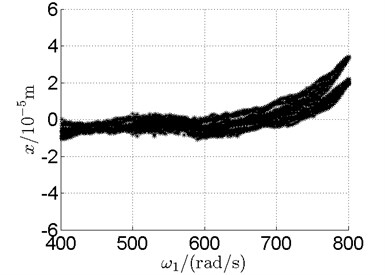
Fig. 10 shows bifurcation diagrams for horizontal displacement of disk 2 and disk 4 with rotor speed. Sampling period for the bifurcation diagram is $5\times 2\pi /{\omega }_1$ because the rotational speed ratio of outer and inner rotor is –1.65 and $5\approx$ 1.65×3. The horizontal axes of Fig. 10(a) and (b) are rotational speeds of inner and outer rotor respectively. And the vertical axes are horizontal displacement of disk 2 and disk 4.

Basically, disk 2 and 4 execute multiple period orbital motion with inner rotor operating in 4-390 rad/s, see Fig. 10(a), Fig. 10(b). However, with the increase of rotational speed, a transformation between periodic and chaotic motion can be observed. From 400 rad/s to 600 rad/s, the rotor execute chaotic motion which can be seen from Fig. 10(c), Fig. 10(d) and Fig. 11.

Fig. 10Bifurcation diagrams of the horizontal response of disk 2 and disk 4 with rotor speed

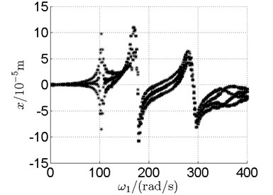
a) Disk 2

b) Disk 4

c) Disk 2

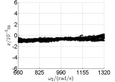
d) Disk 4

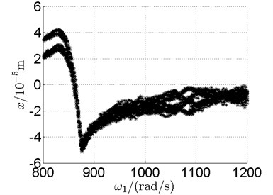
e) Disk 2

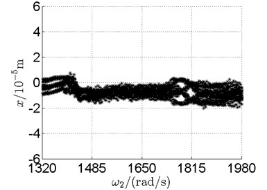
f) Disk 4

g) Disk 2

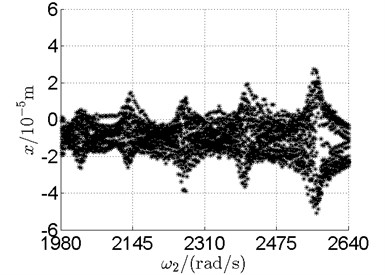
h) Disk 4

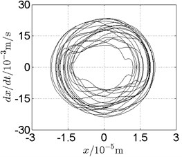
Fig. 11Disk 2: ω1= 500 rad/s, ω2= –825 rad/s

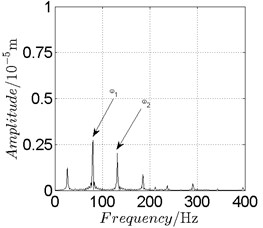
a) Spectrogram

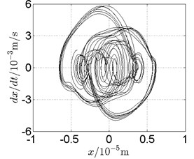
b) Phase trajectory

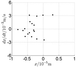
c) Poincare map

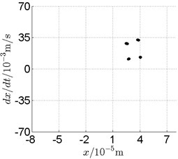
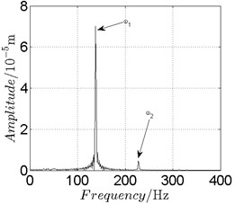
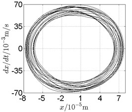
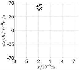
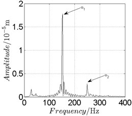
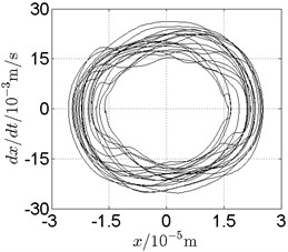
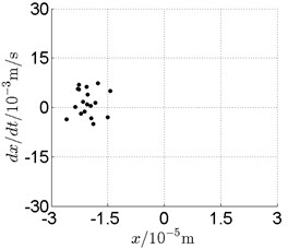
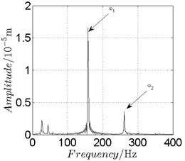
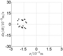
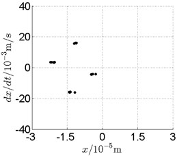
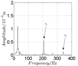
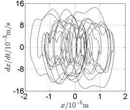
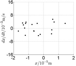
Fig. 12Disk 2: ω1= 740 rad/s, ω2= –221 rad/s

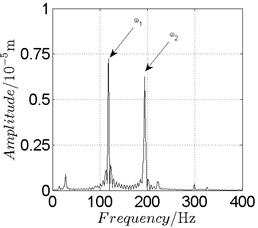
a) Spectrogram

b) Phase trajectory

c) Poincare map

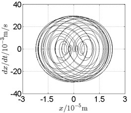
Fig. 13Disk 2: ω1= 820 rad/s, ω2= –1353 rad/s

a) Spectrogram

b) Phase trajectory

c) Poincare map

Fig. 14Disk 2: ω1= 868 rad/s, ω2= –1432 rad/s

a) Spectrogram

b) Phase trajectory

c) Poincare map

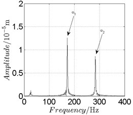
Fig. 15Disk 2: ω1= 950 rad/s, ω2= –1567.5 rad/s

a) Spectrogram

b) Phase trajectory

c) Poincare map

Fig. 16Disk 2: ω1= 990 rad/s, ω2= –1633.5 rad/s

a) Spectrogram

b) Phase trajectory

c) Poincare map

Fig. 17Disk 2: ω1= 1080 rad/s, ω2= –1782 rad/s

a) Spectrogram

b) Phase trajectory

c) Poincare map

Fig. 18Disk 2: ω1= 1300 rad/s, ω2= –2145 rad/s

a) Spectrogram

b) Phase trajectory

c) Poincare map

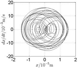
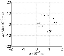
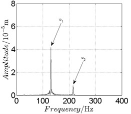
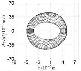
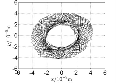
In Fig. 11, continuous spectrum and the disordered discrete points on Poincare map all suggest chaotic motion. With the continuous increasing of rotational speed, from Fig. 12, 740 rad/s for inner rotor, it can be seen that although continuous spectrum still can be observed the discrete points on Poincare map has shown a pattern of surrounding four equilibrium points, which suggests a transformation to periodic motion is undergoing. With higher rotational speed, 820 rad/s, period 4 orbital motion is reached, which can be seen quite obviously from Fig. 10(e), Fig. 10(f) and Fig. 13. Then the process repeats with increasing rotational speeds, see Fig. 10(g), Fig. 10(h) and Fig. 14-Fig. 17.

Besides the pattern of transformation between different states of motion, it is found that the chaotic motion is closely related with the SFD. Fig. 11(a), Fig. 15(a) and Fig. 18(a) show the spectrogram of chaotic motion at different rotational speeds, the same low frequency component, approximately 30 Hz, can be seen quite obviously. This frequency component, 30 Hz or 188 rad/s, is almost the value of the first critical speed excited by the inner rotor. This phenomenon suggests that the SFD has an important influence on the state of motion of the rotor system.

3.3. Experimental validation

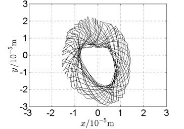
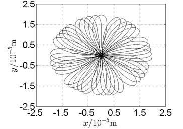
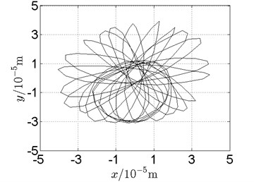
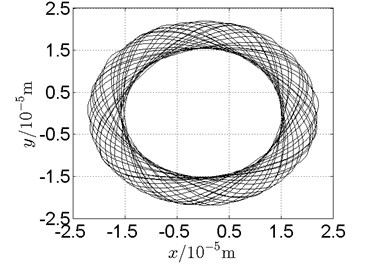
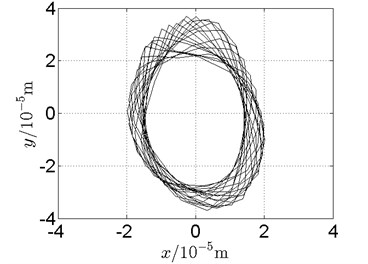
The comparison between numerical and experimental results has already been made in previous section, Fig. 5 and 6. Orbits of disk 2 and 4 under three different rotational speeds are compared in this section for further validation and analysis, see Fig. 19-Fig. 21.

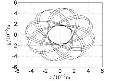
Fig. 19Orbit of disk 2 and disk 4 with ω1= 128 rad/s, ω2= –211 rad/s

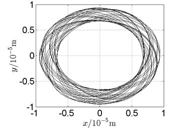
a) Disk 2: numerical results

b) Disk 2: experimental results

c) Disk 4: numerical results

d) Disk 4: experimental results

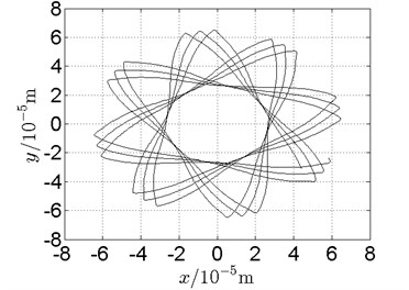
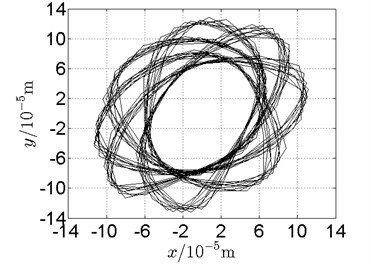
Following conclusions can be reached by analysis of Fig. 19-Fig. 21:

(1) With dual unbalance excitation, disk 2 and 4 execute petal-shaped orbits. Especially when approaching critical speeds of the rotor system, Fig. 20.

(2) The rotor system is slightly anisotropic, which might be caused by the squirrel cage, see Fig. 19(b), Fig. 19(d), 20(b), Fig. 20(d), Fig. 21(b), Fig. 21(d).

(3) Under relatively low speed, the numerical results show great agreement with the experimental results.

Fig. 20Orbit of disk 2 and disk 4 with ω1= 160 rad/s, ω2= –264 rad/s

a) Disk 2: numerical results

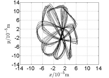
b) Disk 2: experimental results

c) Disk 4: numerical results

d) Disk 4: experimental results

Fig. 21Orbit of disk 2 and disk 4 with ω1= 210 rad/s, ω2= –346 rad/s

a) Disk 2: numerical results

b) Disk 2: experimental results

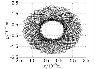
c) Disk 4: numerical results

d) Disk 4: experimental results