Dynamic modelling and control for fully-steerable large reflector antenna considering rigid-flexible coupling

Li, Sulan; Bao, Hong; Wang, Congsi

doi:10.21595/jve.2016.17438

Journal of Vibroengineering

Browse Journal

Submit article

Published: 15 May 2017

Check for updates

Dynamic modelling and control for fully-steerable large reflector antenna considering rigid-flexible coupling

Sulan Li¹

Hong Bao²

Congsi Wang³

^{1, 2, 3}Key Laboratory of Electronic Equipment Structure Design of Ministry of Education, Xidian University, Xi’an 710071, China

Corresponding Author:

Congsi Wang

Cite the article Download PDF

Downloads 1490

Abstract

As the size of reflector antenna increases, the influence of flexible deformation to the system dynamics is much more significant. The coupling between the flexible deformation and the rigid displacement needs to be considered. However, the traditional dynamic modelling and control method for large reflector antenna ignores this coupling. To overcome this problem, this paper proposes a dynamic method based on Lagrange Principle, and the corresponding control strategy is discussed. Finally, we take a 110 m diameter fully-steerable antenna as an example to carry out this method. All the results show that the method is stable and with high precision. It will also lay a solid foundation for the high-precision pointing of large reflector antenna.

1. Introduction

As the most common type of microwave antenna, reflector antenna is used to produce pencil beam to radiate energy towards specified direction, and it has been widely used in space communication, deep space exploration, radio astronomy and other fields [1-6]. In order to explore some unknown territory and capture information from the distant infinite space more effectively, reflector antenna is designed with larger diameter and higher operating frequencies inevitably. If the reflector and feed both can be driven to adjust for pointing according to a certain motion, it is called fully-steerable reflector antenna. At present, the typical fully-steerable reflector antenna contains Green Bank Telescope in American and Effelsberg Telescope in Germany, etc.

With a large reflector, the antenna should be considered as a flexible structure, the influence of low frequency resonant dynamics becomes more significantly [7-10]. So, it is important to establish an accurate overall dynamics model, for improving the closed-loop control performance and the pointing accuracy.

As described above, the overall motion of fully-steerable reflector antennas includes flexible deformation with small amplitude, and rigid displacement with large range in azimuth and elevation direction, respectively. Moreover, they interplay each other. Up to now, the research on dynamic modeling for large reflector antenna has achieved rich fruits. Paper [11] presents the development of the analytical model of the antenna. First, a rigid antenna model is discussed. Next, the modal model of a flexible antenna structure is analyzed based on the finite element data. This analytical model is mainly used in the design stage of the antenna. But the rigid term and flexible term are considered separately, the sum of their linear superposition is taken as output [12, 13]. And for the controlling, paper [14, 15] investigates the relationships between the antenna performance parameters and PI controller gains. It does this for an idealized (or rigid) antenna, and extends the relationships to the NASA Deep Space Network antennas (flexible structures with dish sizes of 34 or 70 meters). It has been noted that the bandwidth, the speed of the system’s response of the PI controller improve with the increase of the controller’s proportional gain, up to a limiting value at which the antenna vibrates. So, the linear quadratic Gaussian (LQG) controller is used for antenna, the performance improves significantly. Paper [16] investigates the LQG controller in detail, including properties, limits of performance, and tuning procedure. Paper [17, 18] investigates the PI controller and $H_{\infty}$ controller. The simulation results show that the performance of $H_{\infty}$ controller is outstanding, but at present, it cannot be implemented because the existing antenna drives operate under acceleration limits that would effectively cancel out the benefits of an $H_{\infty}$ controller. These limits are applied to prevent overloading of the motors. Another typical dynamic modeling method for large reflector antenna [19, 20] is based on system identification principle, and the input and output date are needed. But this method is only suitable for the antenna that has been built on, and not applicable in design stage.

Summarize above, for the dynamic modeling and control of large antenna, there are two problems: 1) for the overall dynamics, the rigid term and flexible term are considered separately, and the coupling between them is not considered, that is not suitable. 2) The controllers are also designed based on the linear superposition dynamics. In this paper, the coupling between the rigid displacements with the flexible deformation will be considered in the dynamic modeling and the control.

The rest of this paper is organized as follows: In Section 2, the modeling and control method considering coupling between the rigid displacements with flexible deformation are proposed. In Section 3, the numerical simulation for 110 m-diameter fully-steerable antenna and experiment verification are given. And conclusions are presented in Section 4.

2. Modeling and control method

The pointing of antenna is codetermined by reflector (primary reflector, and some antenna also contain sub reflector) and feed. In the subsequent analysis, suppose the feed and sub reflector (if it has) is ideal, that is to say, there is no deformation for the sub reflector and feed. The deformation of primary reflector is the main factors to reflect the pointing. In contrast with primary reflector [21], the pedestal is generally designed with higher stiffness, and can be seen as rigid body. Due to the orthogonality between the azimuth axis and elevation axis, the dynamic modeling and the control can be considered individually, and the elevation direction is discussed here.

By introducing the technology of coordinates’ condensation, the flexible deformation is described in modal space in order to reduce the degrees of freedom. So, the modes selection is a key issue. If the number of modes selected is too much, not only a lot of computing time will be spent, but also the controller design based on this model will be very complex and difficult. On the contrary, little modes will lead to large error and low accuracy. Therefore, in order to ensure the accuracy and reliability, it is necessary to study how to select modes.

2.1. Modes selection method

All components of primary reflector should be assembled together, and can be seen as a super unit, and then the key modes are selected based on the modal analysis results.

Let $N$ be a number of degrees of freedom of the system (linearly independent coordinates describing the super unit), $S$ be a number of inputs, $C$ be a number of outputs. The super unit can be represented by the following equation:

1

\{\begin{array}{l} M \ddot{X} + D \dot{X} + K X = B u, \\ y = C X, \end{array}

where $X$ , $\dot{X}$ and $\ddot{X}$ are the nodal displacement, velocity and acceleration vector with the dimension $N \times 1$ , respectively. $u$ is the input vector, $S \times 1$ ; $y$ is the output vector, $C \times 1$ . The mass, stiffness and damping matrix is expressed as $M$ , $K$ and $D$ with dimension $N \times N$ , separately. They are the inherent character of the super unit, the mass matrix is positive definite (all its eigen-values are positive), and the stiffness and damping matrices are positive semi-definite (all their eigen-values are nonnegative). $B$ is the input matrix, and it is determined by the position of the input node of the super unit. $C$ is the output displacement matrix, and it is determined by the position of the output node of the super unit.

$M$ and $K$ can be obtained by assembling the mass matrix and stiffness matrix of each element, respectively. It is difficult to describe the energy dissipation mechanism of the structure exactly, so the true damping characteristics of the structural system is hard to determine accurately, Rayleigh damping [22] is usually assumed as below:

2

D = α_{1} K + α_{2} M .

In order to obtain the modal model, the displacement vector $X$ can be expressed in modal coordinates as following:

3

X (t) = \sum_{i = 1}^{N} \{ϕ_{i}\} q_{i} (t) .

In which, $ϕ_{i}$ and $q_{i}$ are the $i$ th mode shape and mode coordinate, respectively:

4

Φ = [\begin{array}{l} ϕ_{1} & ϕ_{2} & \dots & ϕ_{N} \end{array}] = [\begin{array}{l} ϕ_{1,1} & ϕ_{2,1} & . . . & ϕ_{N, 1} \\ ϕ_{1,2} & ϕ_{2,2} & . . . & ϕ_{N, 2} \\ . . . & . . . & . . . & . . . \\ ϕ_{1, N} & ϕ_{2, N} & . . . & ϕ_{N, N} \end{array}] .

And the $i$ th mode frequency is expressed as $w_{i}$ . In general, with the increasing of mode order $i$ , the corresponding energy of each mode $J_{i}$ decreases, but the sum increases, and the maximum value $J (N)$ is as following:

5

J (N) = \sum_{i = 1}^{N} J_{i}, J_{i} = \frac{1}{2} (k_{i} q_{i}^{2} + m_{i} {\dot{q}}_{i}^{2}) .

If the mode number reaches to a certain value $n$ , the difference between $J (n)$ and $J (N)$ is within an allowable range, then the set of whole modes $N$ would be replaced with the first $n$ modes ( $1 \leq n \leq N$ ).

Note that the modal representation of structure is a set of uncoupled equations. Based on Eq. (1) and Eq. (3), after several equivalent operations, the state space equation for the $i$ th mode can be written as:

6

\{\begin{array}{l} {\dot{x}}_{i} (t) = A_{i q} x_{i} (t) + B_{i q} u_{i} (t), \\ y_{i} (t) = C_{i q} x_{i} (t) . \end{array}

In which, $x_{i} (t) = {(\begin{array}{l} q_{i} (t) & {\dot{q}}_{i} (t) \end{array})}^{T}$ is the $i$ th state vector ( $1 \leq i \leq n$ ), $q_{i} (t)$ is the $i$ th modal coordinate as described above, ${\dot{q}}_{i} (t)$ is the $i$ th modal velocity coordinate. $A_{i q}$ is the system matrix, it is determined as follows:

7

A_{i q} = [\begin{matrix} 0 & 1 \\ - w_{i}^{2} & - 2 ς_{i} w_{i} \end{matrix}],

where $ς_{i}$ is the $i$ th modal damping ratio. For Rayleigh damping, the damping ratio and frequency have the following relationship [22]:

8

ζ_{n} = \frac{α_{1}}{2 Ω_{n}} + \frac{α_{2} Ω_{n}}{2} .

Details of how the damping ratio varies with frequency are scarcely available. It is usually assumed that the damping ratio applied to each frequency is the same, that is, the equivalent damping ratio with the same attenuation rate is used to express the damping of the actual structure. Although this is a special case, in practical applications, the damping of the vibration system is generally small, the equivalent method can be found in the well-known antenna dynamics modeling [11-18].

And $B_{i q}$ , $C_{i q}$ is the input and output matrix, respectively:

9

B_{i q} = Φ^{T} B,

10

C_{i q} = C Φ .

Theoretically, the determination of them requires large matrix $Φ$ . In fact, one needs only one column/row of it for each input/output matrix as the input matrix $B$ is composed of zero, except the location of the actuator (pinion) of structure. The same is output matrix $C$ , which is also of all zero, except the location of the sensor (encoder) of structure.

Based on the above state space equation, the corresponding transfer function is obtained according to the modern control theory [23]:

11

G_{i} (w) = C_{i q} {(j w I - A_{i q})}^{- 1} B_{i q}, \begin{array}{l} (i = 1,2 \dots, n) \end{array} .

And its $H_{2}$ norm is as following:

12

{‖G_{i} (w)‖}_{2} = {‖C_{i q} {(j w I - A_{i q})}^{- 1} B_{i q}‖}_{2} \begin{array}{l} , & (i = 1,2, \dots, n), \end{array}

where $I$ is identify matrix, $j = \sqrt{- 1}$ . The norm reflects the contribution of each mode to the system output. Since each mode is independent, therefore, the $H_{2}$ norm of the transfer function describing the reflector structure is approximately the RMS (Root Mean Square) of the modal modes norms:

13

{‖G (w)‖}_{2} = \sqrt{\sum_{i = 1}^{n} {‖G_{i} (w)‖}_{2}^{2}} .

The ratio of each mode:

14

η_{i} = {‖G_{i} (w)‖}_{2} / {‖G (w)‖}_{2} .

In accordance with this ratio, arrange the state variables in descending order. The states with the smallest $H_{2}$ are the last ones in the arrangement. Truncate the least important states, suppose $k$ is the remained number, this number is determined according to the truncating error in following:

15

e_{2} = {(\sum_{i = k + 1}^{n} {‖G_{i} (w)‖}_{2})}^{\frac{1}{2}} .

The remained number is enough that the truncating error satisfies the requirement, it means that the remaining states represent the significant portion of the antenna structural dynamics.

2.2. Description of super unit

The generalized coordinates to describe the super unit is as follows:

16

ξ = \{\begin{array}{l} p \\ ϑ \\ q \end{array}\} = \{\begin{matrix} x \\ y \\ z \\ ϕ \\ φ \\ θ \\ q_{i}, i = 1, \dots k \end{matrix}\},

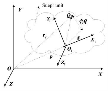
$p = (\begin{array}{l} x & y & z \end{array})$ is the Cartesian coordinate in the global system of the super unit, $ϑ = (\begin{array}{l} ϕ & φ & θ \end{array})$ is the Euler angles to reflect the orientation for this super unit, $q = (\begin{array}{l} q_{1}, & q_{2}, & \dots, & q_{k} \end{array})$ is the modal coordinates. As shown in Fig. 1, $O X Y Z$ is the global coordinate system, $O_{1} X_{1} Y_{1} Z_{1}$ is the local coordinate system, the position vector of node $Q$ of this super unit in global system can be expressed as:

17

r_{i} = p + T (s + ϕ_{i} q) .

where $r_{i}$ is the vector of node $Q$ in global system; $p$ is the origin vector of local coordinate system in global coordinate system; $T$ is the transformation matrix from local coordinate system $O_{1} X_{1} Y_{1} Z_{1}$ to the global coordinate system $O X Y Z$ ; $s$ is the coordinate of nodes in local coordinate system before deformation; $ϕ_{i}$ is the modal matrix corresponding to the node, and $q$ is the modal coordinates.

Fig. 1Position of node on super unit

From Eq. (17), it can be seen that the movement of super unit can be decomposed into three parts such as: rigid movement, rigid rotation and flexible deformation. The speed of this node can be obtained by derivation for the above expression:

18

v_{i} = \frac{d r_{i}}{d t} = \frac{d p}{d t} + \frac{d T}{d t} (s + ϕ_{i} q) + T \frac{d (s + ϕ_{i} q)}{d t} .

2.3. Dynamic modeling based on Lagrange equation

Taking Eqs. (17-18) into the following equation, the kinetic energy of super unit can be obtained:

19

K_{1} = \frac{1}{2} \int ρ v_{i}^{T} v_{i} d V,

where $ρ$ is the density of super unit. And potential energy specifically includes gravitational potential energy and elastic potential energy:

20

P_{1} = \int ρ g d V + \frac{1}{2} \int {(ϕ_{i} q)}^{T} K ϕ_{i} q d V .

Combined with the kinetic and gravitational potential energy of pedestal, the dynamic equations would be obtained according to the Lagrange principle:

21

\frac{d}{d t} \frac{\partial K}{\partial \dot{κ}} - \frac{\partial K}{\partial κ} + \frac{\partial P}{\partial κ} = Q,

where, $K$ is the total kinetic energy, $P$ is the total potential energy, $κ$ is the generalized coordinate, and $Q$ is generalized torque.

2.4. Controller design

Based on the above dynamic modeling, in the following, the controller design will be discussed. Considering that the movement in azimuth and elevation direction is independent, and their dynamic model and controller are independent as well, so only the controller in elevation direction is taken as an example to illustrate this problem. The diagram is shown in Fig. 2.

Fig. 2Antenna control system

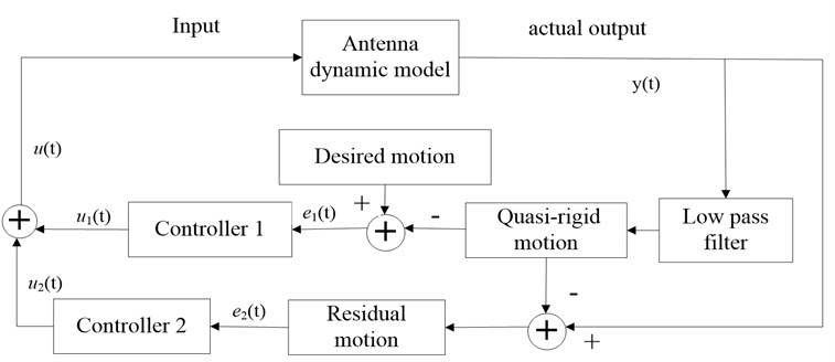
As described above, except rigid displacement, the actual output also includes flexible deformation and the rigid-flexible coupling terms. So, a low pass filter which is described as follows is used:

22

G (j w) = \frac{1}{1 + \frac{\sqrt{2} j w}{w_{c}} + {(\frac{j w}{w_{c}})}^{2}},

where $w_{c}$ is the cut-off frequency of the filter, it is determined by:

23

w_{c} = c_{1} 2 π f_{1},

where $c_{1}$ is a scale factor, and satisfies $0 \leq c_{1} \leq 1$ , it can be adjusted according to actual situation; $f_{1}$ is the lowest frequency in the modal selecting process. Different scale factor $c_{1}$ corresponding to different output of low pass filter. Here, it is regarded as quasi-rigid displacement as rigid displacement is in large proportion of this signal. And the residual terms contain most of the flexible deformation and other coupling terms.

Based on the PID control principle, two specially designed controllers in figure 1 will be introduced in the following. Controller 1 is used for $e_{1} (t)$ in order that the quasi-rigid displacement may consistent with the desired motion, and controller 2 is used for $e_{2} (t)$ in order to suppress the residual deformation. Considering that, there is large error when the antenna is in the start or stop stage, and the accumulation of error may lead to $u_{1} (t)$ exceeding the maximum amount allowed by the servo motor, and causing large overshoot or oscillation. So, integral coefficient variable PID is used, and its discrete form is shown as following:

24

u_{1} (k) = k_{p 1} e (k) + k_{i 1} (\sum_{i = 0}^{k - 1} e (k) + f (e (k)) e (k)) + k_{d 1} (e (k) - e (k - 1)) .

In which, $k_{p 1}$ , $k_{i 1}$ , $k_{d 1}$ is the proportional, integral and differential coefficient, respectively. The determination of $f (e (k))$ is shown as following:

25

f (e (k)) = \{\begin{array}{l} 1, |e (k)| \leq B, \\ \frac{A - |e (k)| + B}{A}, B < |e (k)| \leq A + B, \\ 0, |e (k)| > A + B, \end{array}

where $e (k)$ is the current error, $f (e (k))$ varies between [0, 1]. Parameter $A$ determines the rate of varying from 1 to 0, the greater the value of $A$ , the slower the rate of $f (e (k))$ varying; and parameter $B$ determines the length of time to take for maximum value 1. The determination of $A$ , $B$ are related to $e (k)$ . In order to prevent integral saturation, and ensure the rapidity of response, it usually can be considered that $A = 0.3 m a x (e (k))$ , $B = 0.5 m a x (e (k))$ firstly, then according to the response adjust these two parameters. It can be seen from Eq. (25). This is a relatively slow method to adjust the integral term depending on the current error.

Controller 2 is designed to suppress the residual vibration, and there are some high frequency components in $e_{2} (t)$ . The presence of differential term is not beneficial to the stability of the system, so PI controller is used:

26

u_{2} (t) = k_{p 2} e (t) + k_{i 2} \int e (t) d t,

where $k_{p 2}$ , $k_{i 2}$ is the proportional and integral gain coefficient, individually.

3. Simulations and experiment

3.1. The antenna description

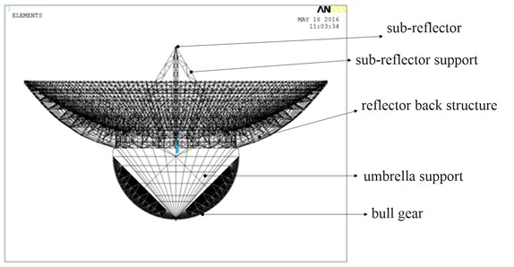
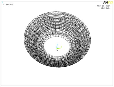
The proposed method is used for a 110 m-diameter fully-steerable antenna as shown in Fig. 3, which is planned to be built in XinJiang Province in China [24]. The reflector is considered as flexile body, and its finite element model is shown in Fig. 4.

In Fig. 4, the bull gear is modeled using 206 shell63 elements. Sub-reflector, counter weight and feed are equivalent to mass element attached to the corresponding hanging nodes, there are 3954 mass21 elements. And 16308 beam188 elements are used for other support structure.

Fig. 3110 m-diameter fully-steerable antenna CAD model

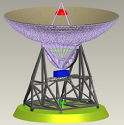
Fig. 4Finite element model of reflector

The back structure is of typical rotational symmetry. Its single-chip radial beam is shown in Fig. 5, which is composed of the around beam, bottom beam, web girder and short beam between around beam and web girder. Between the two adjacent radial beams, there is a parallel beam structure and a number of slanting beams to improve the stiffness of the structure.

Fig. 5Finite element model of back structure

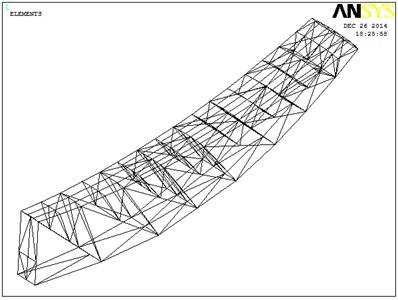
a) Single-chip radial beam

b) Reflector back structure

For simulating the engagement of bull gear and pinion, the pinion is modeled using beam element, as shown in Fig. 6, and the end of the beam which is not connected with the gear is fully constrained. The pinion radius is $r_{1}$ , a torque $T$ applied at the pinion of the gearbox is the input to the structure. A node labeled $n_{0}$ in the finite element model is a point of contact between the pinion and the bull gear. The torque $T$ applied to the pinion is in equilibrium with tangential (to the bull gear and the pinion) force $F_{n_{0}}$ , for the force with $y$ and $z$ components:

27

F_{n 0} = [\begin{array}{l} F_{0 y} \\ F_{0 z} \end{array}] = [\begin{array}{l} F_{n 0} s i n α \\ F_{n 0} c o s α \end{array}] = [\begin{array}{l} \frac{T s i n α}{r_{1}} \\ \frac{T c o s α}{r_{1}} \end{array}] = [\begin{array}{l} \frac{s i n α}{r_{1}} \\ \frac{c o s α}{r_{1}} \end{array}] T .

The absolute value, one obtains from Fig. 6.

Fig. 6Engagement of bull gear and pinion

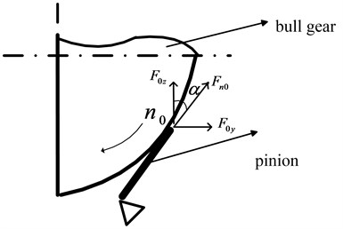
Then, according to Eq. (7):

28

B_{i q} = {Φ_{i}}^{T} {[\begin{array}{l} 0 & \dots & 0 & 0 & s i n α / r_{1} & c o s α / r_{1} & 0 & \dots \end{array}]}^{T} .

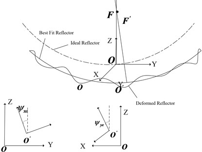
In Fig. 7, the pointing of ideal antenna is described with $\vec{O F}$ (normal vector of designed ideal reflector), and the pointing of antenna with flexible deformation is represented by $\vec{O^{'} F^{'}}$ (normal vector of best fit surface for deformed reflector). The angle between these two vectors is the pointing error angle. In the following, the projection of this angle on $X O Y$ plane and $Y O Z$ plane corresponds to azimuth angle error and pitch angle error. The angle error can be determined using the Best-Fit-Paraboloid (BFP) method as following:

29

[\begin{array}{l} ψ_{x e} \\ ψ_{y e} \end{array}] = \frac{1}{f} [\begin{array}{l} 0 & 0 & 0 & 0 & 1 & 0 \\ 0 & 0 & 0 & 0 & 0 & 1 \end{array}] S T P \cdot X_{r} = C \cdot X_{r},

where $f$ is the focal length, $S$ , $T$ , $P$ are all determined by the BFP method, $X_{r}$ is the displacement matrix of nodes in reflector. Then according to Eq. (8), $C_{i q}$ can be obtained.

Fig. 7Pointing of reflector

3.2. Modal selection

Based on the modal analysis of the above structure, the first 8 order natural frequencies are shown in Table 1.

According to previous section, $A_{i q}$ , $B_{i q}$ , $C_{i q}$ can be determined, the $H_{2}$ norm for each mode based on Eq. (9) are computed as shown in Fig. 8.

Table 1Frequency of the reflector

Order	1	2	3	4	5	6	7	8
Frequency	$f_{1} =$ 0.6257	$f_{2} =$ 1.6591	$f_{3} =$ 1.6611	$f_{4} =$ 1.7877	$f_{5} =$ 1.8278	$f_{6} =$ 1.8663	$f_{7} =$ 1.8814	$f_{8} =$ 1.9907

Fig. 8H2 Norm and the 1st mode deformation

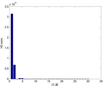
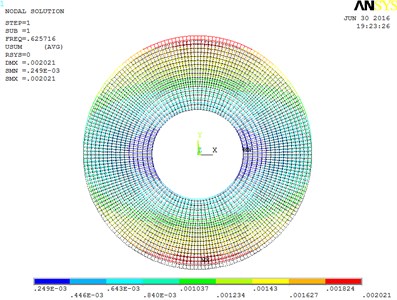
Take the truncating error satisfying $e_{2} \leq$ 0.001. The 1st, 2th and 5th order modes are selected. Although the absolute energy of the 3rd and 4th mode is larger than the order behind it, but it is the twisting motion about the focal axis, and does not lead to pointing error. So, the $H_{2}$ norm is smaller than the 5th mode, and not selected. Other modes are rejected as they are the local vibration of umbrella support, and with little effect to the pointing error.

The average computing time of impulse response, before and after the modes selection, with the same computer (3.4 GHz, I3-2130 CPU and 2GB of computer memory) are shown in Table 2.

The steady state value and error of impulse response are shown in Table 3.

Table 2Average computing time

Output	Before/s	After/s	Percentage saving time
Elevation error angle	0.2035584	0.067432	66.8 %
Azimuth error angle	0.2327347	0.075436	67.6 %

Table 3Impulse response

Output	Steady value / rad	Steady error / rad	Relative error
Elevation error angle	8.963421×10^-14	–4.439763×10^-15	4.95 %
Azimuth error angle	9.594521×10^-16	5.253912×10^-1)	5.47 %

From the above results, it can be seen that, the relative steady state error is less than 6 %, but the computation time is greatly reduced. The mode selection method is effective.

3.3. Dynamical simulations and control

In order to verify the correctness of the dynamic model, establishing an ideal antenna (all of the components are rigid) dynamic model. As in practice, the antenna rotates always with very slow start and stop. So, driven torque as shown in Fig. 9(a) is applied in the following simulation, Fig. 9(b) shows the corresponding angular velocity. In these figures, blue line indicates amount in azimuth direction, and dashed line indicates ideal antenna, solid line indicates actual antenna. The angular displacement and acceleration both can be obtained.

Fig. 9Dynamic output

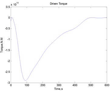
a) Driven torque

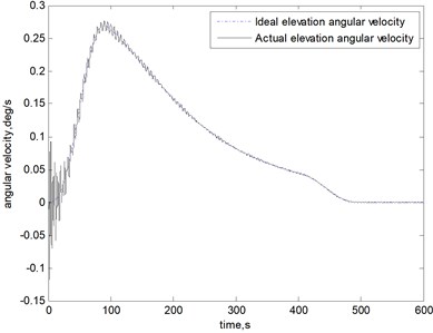
b) Angular velocity

It can be seen that, during the movement, the trend of elevation angular velocity output is consistent with the ideal antenna, but is accompanied by high frequency vibration. The amplitude is about 0.005 deg/s. It has great impact on the stability and reliability of the antenna, and the pointing accuracy will also be certainly lost. Therefore, in the following of the controller design, the flexible vibration needs to be suppressed as much as possible. According to the angular velocity, the angular displacement and acceleration both can be obtained.

3.4. Controller simulation

In this section, the purpose is to adjust the control torque to make the antenna track the required target with the controller designed as shown in Fig. 2. Additionally, the requirement for QTT is also considered for this design, the maximum angular velocity in elevation direction is 0.3 deg/s, and the maximum angular acceleration is 0.15 deg/s².

A traditional single PID controller is designed to contrast with the above PID controller. All of the parameters, including the scale factor of filter, and the gains of PID controller, are determined by optimizing according to the specify performance index. The results are shown as following. The dashed line corresponds to the performance of the proposed method in this paper, while the solid line corresponds to the single PID method.

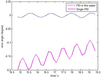
From Fig. 10, it can be seen that: compared with single PID controller, the performance of the controller presented in this paper are both better than the single PID. The settling time for single PID method is 27.3 s, while for the PID in this paper is 12.45 s, it is shorter by 54.6 %. In order to reflect the effect more clearly, the comparison of track error is shown in Fig. 11, the steady state errors are 0.0016 deg/s and 0.018 deg/s, respectively. The amplitude of the vibration decreases. It is due to separate the quasi-rigid signal with the flexible vibration signal using a filter. Compared with single PID method, there are more adjustable gain parameters for the PID method in this paper, the dimensions of the corresponding design space are larger, so better performance will be gotten. On the other hand, the computational cost increases, and the torque required is much greater, so higher performance will be required for servo motor.

$e_{1} (t)$ , $e_{2} (t)$ are the input of controller 1 and controller 2, respectively. $u_{1} (t)$ , $u_{2} (t)$ are the output correspondingly. Considering rigid-flexible coupling, $e_{1} (t)$ , $e_{2} (t)$ are not independent each other. So, adjusting the gain of one of the controllers affects not only the output of this controller, but also the performance of the other controller. Here the relationship between the signals is analyzed using the theory of correlation function. The cross correlation function is used to describe the correlation statistics between two different signals, its numerical expression is showed as follows:

30

R_{f 1, f 2} (l) = \frac{1}{N} \sum_{k = 0}^{N} f_{1} (k) f_{2} (k + l),

where $N$ is the number of points, $l$ is the interval. And the corresponding cross correlation coefficient is defined as:

31

c_{f 1, f 2} = \frac{\sum_{k = 0}^{N} f_{1} (k) f_{2} (k + l)}{{(\sum_{k = 0}^{N} f_{1} (k) f_{1} (k + l))}^{0.5} {(\sum_{k = 0}^{N} f_{2} (k) f_{2} (k + l))}^{0.5}} .

Fig. 10Dynamic output

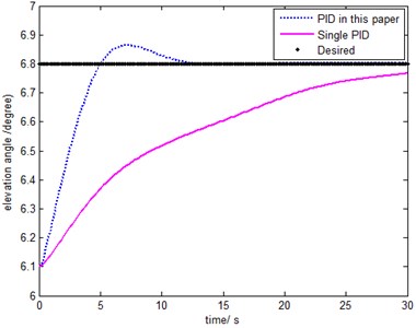
Fig. 11Error angle

If $c_{f 1, f 2} = 0$ , then the corresponding signals $f_{1} (t)$ , $f_{2} (t)$ are uncorrelated. If $c_{f 1, f 2} =$ ±1, then the two signals are perfectly correlated.

So according to the above theory, and combining the numerical calculation results, compute the correlation coefficients as following:

32

c_{y, e 1} = 0.8792, c_{y, e 2} = 0.0463, c_{e 1, e 2} = 0.1926 .

From these results, it is clear that the correlation between the actual output of the antenna and the quasi-rigid error is much larger than that between the actual ouput and the residual deformation, and also there is some relationship between the quasi-rigid error and the residual deformation. It all shows that the coupling of rigid and flexible does exist and cannot be ignored.

3.5. Experimental verification

As QTT has not yet been built, and is still at the design stage. An experiment is designed to validate the above control method as following. The equipment is depicted in Fig. 12. The main objective of this experiment is to control the position of the flexible link’s tip using the above method, and analyze the simulation and experimental results.

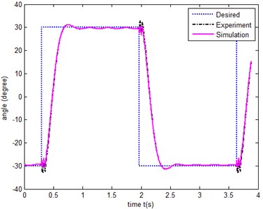
The purpose is to adjust the control torque to make the flexible link track the required rectangular square wave with an amplitude of 30 degrees, and a frequency of 0.3 Hz. using the PID presented in Section 2.4, the results of simulation and experiment are showed in Fig. 13.

Fig. 13 depicts that the simulation results and experimental results are basically consistent, the simulation of controllers designed is with good performance, and there is little slight oscillation when the amplitude of the rectangular wave verifies. Compared with the simulation results, the experimental result shows it is always with larger oscillation. It is due to the fact that the conditions of the simulation are ideal, and there may be more interference in the experiment.

Fig. 12SRV02-flexible link

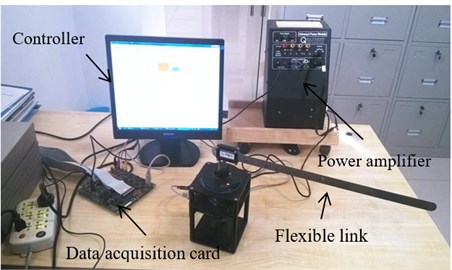
Fig. 13Results contrast

4. Conclusions

With the increasing of antenna diameter, rigid motion assumption may be not accurate, and it is also not suitable for linear superposition of flexible deformation with rigid displacement. To deal with above problems for large fully steerable antenna, this paper presents the corresponding modeling and control method. All components of primary reflector are assembled together which can be seen as a super unit, then based on Lagrange Principle the dynamic model of the reflector antenna is deduced. In view of the characteristics of this model, two special controllers are designed. Lastly, all of the simulation and experimental results show that the system modeling and control method are effective and reliable.

References

Rahmat-Samii Yahya, Densmore Arthur C. Technology trends and challenges of antennas for satellite communication systems. IEEE Transactions on Antennas and Propagation, Vol. 63, Issue 4, 2015, p. 1191-1204.

Publisher
Rao Sudhakar K. Advanced antenna technologies for satellite communications payloads. IEEE Transactions on Antennas and Propagation, Vol. 63, Issue 4, 2015, p. 1205-1217.

Publisher
Duan Baoyan Study on optimization of mechanical and electronic synthesis for the antenna structural system. Mechatronics, Vol. 4, Issue 6, 1994, p. 553-564.

Publisher
Deng Bin, Wang Hongqiang, Qin Yuliang, et al. Rotating parabolic-reflector antenna target in SAR data: model, characteristics, and parameter estimation. International Journal of Antennas and Propagation, Vol. 2013, 2013, p. 583865.

Publisher
Li Bing, Qi Xiaozhi, Huang Hailin, et al. Modelling and analysis of deployment dynamics for a novel ring mechanism. Acta Astronautica, Vol. 120, 2016, p. 59-74.

Publisher
Duan Xuechao, Qiu Yuanying, Bao Hong, et al. Real time motion planning based vibration control of a macro micro parallel manipulator system for super antenna. Journal of Vibroengineering, Vol. 16, Issue 2, 2014, p. 694-703.

Search CrossRef
Duan Baoyan, Wang Congsi Reflector antenna distortion analysis using MEFCM. IEEE Transaction of Antennas and Propagation, Vol. 57, Issue 10, 2009, p. 3409-3413.

Publisher
Asbrri Polo, Sabatini Marco, Pisculli Andrea Dynamic modelling and stability parametric analysis of a flexible spacecraft with fuel slosh. Acta Astronautica, Vol. 127, 2016, p. 141-159.

Publisher
Wang Zhaohui, Jia Yinghong, Xu Shijie, et al. Active vibration suppression in flexible spacecraft with optical measurement. Composite Structures, Vol. 55, 2016, p. 49-56.

Publisher
Bin DiYou, Jian Minwen, Yang Zhao Nonlinear analysis and vibrations suppression control for a rigid-flexible coupling satellite antenna system composed of laminated shell reflector. Acta Astronautica, 2014, p. 269-279.

Publisher
Gawronski Wodek Modeling and Control of Antennas and Telescopes. Springer, Germany, 2008.

Publisher
Gawronski Wodek, Mellstrom J. A. Elevation Control System Model for the DSS 13 Antenna. TDA Progress Report 42-105, 1991, p. 83-85.

Search CrossRef
Gawronski Wodek, Mellstrom J. A. Modeling and Simulations of the DSS 13 Antenna Control System. TDA Progress Report 42-106, 1991, p. 205-248.

Search CrossRef
Gawronski Wodek, Mellstrom J. A. Antenna servo design for tracking low-earth orbit satellites. AIAA Journal of Guidance, Control Dynamics, Vol. 17, Issue 6, 1994, p. 1179-1184.

Publisher
Gawronski Wodek Servo performance parameters of the NASA Deep space network antennas. IEEE Antennas and Propagation Magazine, Vol. 49, Issue 6, 2007, p. 40-46.

Publisher
Gawronski Wodek Antenna linear quadratic-Gaussian (LQG) controllers: properties, limits of performance, and tuning procedure. Caltech, JPL, Technical Report 42-158, Pasadena, CA, USA, 2004, p. 1-18.

Search CrossRef
Gawronski Wodek Antenna control systems: from PI to H∞. IEEE Antennas and Propagation Magazine, Vol. 43, Issue 1, 2001, p. 52-60.

Publisher
Gawronski Wodek Design and performance of the H∞ controller for the beam-waveguide antennas. IPN Progress, Report 42-184, 2011, p. 1-22.

Search CrossRef
Landau Identification in closed loop: a powerful design tool (better design odels, simpler controllers). Control Engineering Practice, Vol. 9, 2001, p. 51-65.

Publisher
Gawronski Wodek Advanced Structural Dynamics and Active Control of Structures. Springer, New York, 2004.

Publisher
Huang Yaude, Raffin Philippe, Chen Mingtang Stiffness study of a Hexapod telescope platform. IEEE Transactions on Antennas and Propagation, Vol. 59, Issue 6, 2011, p. 2022-2028.

Publisher
Clough R. W., Penzien J. Dynamics of Structures. Second Edition, Higher Education Press, Beijing, 2006.

Search CrossRef
Skogestad S., Postlethwaite I. Multivariable Feedback Control: Analysis and Design. John Wiley and Sons, New York, 2005.

Search CrossRef
Wang Na Xinjiang Qitai 110 m Radio Telescope. Scientia Sinica Physica, Mechanica and Astronomica, Vol. 44, Issue 8, 2014, p. 783-794.

Publisher

About this article

Received

21 July 2016

Accepted

15 December 2016

Published

15 May 2017

SUBJECTS

Vibration generation and control

DOI

https://doi.org/10.21595/jve.2016.17438

Keywords

reflector antenna

dynamic model

flexible deformation

Lagrange equation

control

Acknowledgements

This project was supported by National Natural Foundation of China (No. 51305321), National Key Basic Research Program 973 (No. 2015CB857100). These supports are gratefully acknowledged. Many thanks are due to the editors and reviewers for their informative, valuable and constructive comments.

This is an open access article distributed under the Creative Commons Attribution License, which permits unrestricted use, distribution, and reproduction in any medium, provided the original work is properly cited.

Previous article in issue Previous Next article in issue Next

Research article

2023 10 31

Rigid-flexible coupling modeling of the dual-rotor system for aero-engine

Pingping Ma, Yuehui Dong, Hangqi Zhao, Yang Li, Muge Liu

Research article

2020 11 05

Distributed vibration control for large-scale flexible space structure improved by fuzzy logic system

Xiang Wang, Xiaoyu Wang, Hongyou Chai

Research article

2020 08 15

On dynamics of a rotating hub-flexible rod-concentrated mass system considering rigid-flexible coupling effect

Jianshi Fang, Jianqiang Xiao, Liang Li, Dingguo Zhang

Research article

2018 03 31

A more accurate dynamic model for dual-side excitation large vibrating screens

Liping Peng, Runxin Fang, Huihui Feng, Lei Zhang, Wenda Ma, Xiaodi He

S. Li, H. Bao, and C. Wang, “Dynamic modelling and control for fully-steerable large reflector antenna considering rigid-flexible coupling,” Journal of Vibroengineering, Vol. 19, No. 3, pp. 1867–1881, May 2017, https://doi.org/10.21595/jve.2016.17438

Copy Extrica

Copied to clipboard!

TY  - JOUR
DO  - 10.21595/jve.2016.17438
UR  - https://doi.org/10.21595/jve.2016.17438
TI  - Dynamic modelling and control for fully-steerable large reflector antenna considering rigid-flexible coupling
T2  - Journal of Vibroengineering
AU  - Wang, Congsi
AU  - Li, Sulan
AU  - Bao, Hong
PY  - 2017
DA  - 2017/05/15
PB  - JVE International Ltd.
SP  - 1867-1881
IS  - 3
VL  - 19
SN  - 1392-8716
ER  - 

Copy Ris

Copied to clipboard!

@article{Wang_2017,
	doi = {10.21595/jve.2016.17438},
	url = {https://doi.org/10.21595/jve.2016.17438},
	year = 2017,
	month = {may},
	publisher = {{JVE} International Ltd.},
	volume = {19},
	number = {3},
	pages = {1867--1881},
	author = {Congsi Wang and Sulan Li and Hong Bao},
	title = {Dynamic modelling and control for fully-steerable large reflector antenna considering rigid-flexible coupling},
	journal = {Journal of Vibroengineering}
}

Copy Bibtex

Copied to clipboard!

[1]C. Wang, S. Li, and H. Bao, “Dynamic modelling and control for fully-steerable large reflector antenna considering rigid-flexible coupling,” Journal of Vibroengineering, vol. 19, no. 3, pp. 1867–1881, May 2017, doi: 10.21595/jve.2016.17438.

Copy IEEE

Copied to clipboard!

Wang, Congsi, Sulan Li, and Hong Bao. “Dynamic Modelling and Control for Fully-Steerable Large Reflector Antenna Considering Rigid-Flexible Coupling.” Journal of Vibroengineering 19, no. 3 (May 15, 2017): 1867–81. https://doi.org/10.21595/jve.2016.17438.

Copy Chicago

Copied to clipboard!

Dynamic modelling and control for fully-steerable large reflector antenna considering rigid-flexible coupling

Abstract

1. Introduction

2. Modeling and control method

2.1. Modes selection method

2.2. Description of super unit

2.3. Dynamic modeling based on Lagrange equation

2.4. Controller design

3. Simulations and experiment

3.1. The antenna description

3.2. Modal selection

3.3. Dynamical simulations and control

3.4. Controller simulation

3.5. Experimental verification

4. Conclusions

References

About this article

Related Articles