Abstract
During driving of a vehicle on road, the tires are undertaking load conversion of the vehicle under various driving conditions and various road conditions within contact patches. As for the contact condition between tire and road, it is often deemed as composed by spring and damping element. The contact with road is always simplified as point contact. Besides, static friction model is adopted, which has ignored physical property of friction and dynamic process of establishment of friction force. It is far from sufficient for current vehicle and road safety design. In this paper, ADAMS software is applied to establish a multi-body dynamics model of heavy vehicle, actual vehicle data was adopted to check virtual sample vehicle, and the Strikbeck dynamical friction property is introduced to tire model during rolling contact between tire and payment, interface of Simulink with ADAMS is applied to put forward a complete vehicle dynamic model truly reflecting the process of dynamic contact between tire and road, and furthermore the correctness and availability of dynamic tire model are verified through comparison with classic Pac2002 tire model. As for dynamic behaviors of heavy vehicle in special sections, finite element method (FEM) is applied to put forward a new 3D complicated road model construction method to construct roads of different classes and long-downhill paths of different S-curves. Simulated analysis of the influence of different speeds, different classes of random roads, different slopes and different adhesion road models on ride comfort of vehicle driving was implemented through utilization of event editor and drive control file, and speed limit standards under different conditions are put forward, so as to provide theoretical basis for road alignment design and reasonable driving speed. Finally, the influence and changing rules of different speeds, different classes of random roads and different slopes on driving safety are discussed from the perspectives of each radial force of tire, alignment torque, sideslip angle and roll angle.
1. Introduction
Load transmission between vehicle and road is realized through tire/road contact patch. The hyperbolic structure of the tire and the large deformation characteristic of rubber material make the contact patch a dynamical boundary. During contact with the road, the tire goes through stretch, compression and bending to adapt top ups and downs of the road so as to generate complicated normal and tangential stress field on the contact interface. The stress distribution depends on wheel load, vehicle driving status, tire structure and tire/road friction status. Greenwood and Williamson (1966) [1] put forward the famous GW contact model and analyzed the contact mechanisms of irregular surfaces with an-isotropic characteristics, thus creating the research field of an-isotropic rough surface contact theories. Gal (2008) [2] described rough contact as micro area (5-100 μm) and macro area (300-1000 μm), established a rough road hysteresis friction factor model in consideration of characteristics of vertical acting force, conducted in-depth research on physical properties of hysteresis friction factor of rubber, and pointed out that the macro area was the main area influencing hysteresis friction factor and actual contact area. Carbone (2009) [3] proposed the improvement of GW model and developed the research of contact theory from micro area to macro area, thus laying a foundation for modeling through introduction of rubber friction to vehicle macro system. Heinrich (2008) [4] studied the mechanism concerning interaction between sliding tire and rough road, analyzed the influence of the energy loss from deformation of tire tread on the sliding friction factor and estimated the dynamic sliding friction factor with sliding area of the tire. Wei (2012) [5] applied Lagrange-Euler mixed description method to analyze speed field, accelerated speed field and contact deformation of tire big-deformation rolling contact structure, used orientation angle of the wheel as Cardan angle, relied on Lagrange description to obtain tire speed field containing rigid body rotation and elastic deformation, used Euler description to obtain deformation and stress of contact area, and completed dynamic analysis of rolling structure through information transmission of Euler network and Lagrange network. Xu (2013) [6] simplified tire/road actual contact area model and viscoelasticity energy loss, established an improved sliding friction factor model and intensively analyzed the action of tire and road characteristics on sliding friction factor. The interaction between tire and road is a very complicated dynamic process. During vehicle braking and turning, the friction status between tire and ground continuously changes. Adhesion friction force (adhesion area) and hysteresis friction force (sliding area) are nonlinear and changing dynamically. Therefore, it is difficult to carry out qualitative and quantitative description. To this end, good tire/road friction model cannot only reasonably express the dynamic behavior during tire/road contact motion but also be easily applied in vehicle control system. Tire/road friction model was classified as semi-empirical model and analytical model [7, 8]. Semi-empirical model can describe steady tire/road friction characteristics in a relatively accurate way since - is usually obtained using curve fitting method based on experimental data. However, this model cannot reflect the influence of surface characteristics of road, tire pressure, hysteresis and other relevant factors on friction characteristics. It is actually a static friction model. Typical semi-empirical models include piecewise linearity model, Burckhardt model, Rill model, Magic model and Karnopp. Differential equation is usually adopted in analytical model to describe tire/road friction characteristics. It is actually a dynamical friction model. Typical analytical models include Armstrong model, Brush model, Dahl model, Bliaman-Sorine model and LuGre model. Abundant researches and application results indicated that LuGre model was the best among all analytical models. LuGre model boasted compact mathematical form and definite physical significance [9-11]. Deura (2004) [12] put forward a three-dimensional dynamical brush model based on LuGre friction model. This new model could simulate dynamical vertical and horizontal friction forces and alignment torques of tire in a relatively favorable way. Zuo Shuguang (2012) [13] established a tire-road finite element model based on LuGre dynamical friction model, conducted simulated analysis on lateral self-induced vibration of tire and research on influencing factors, and pointed out that lateral self-induced vibration would occur to the rolling tire under certain conditions so as to result in polygon abrasion of tire. The lumped LuGre tyre model and the vehicle kinematics are combined, the tyres internal deflection state is used to gain an accurate estimation (2016) [14]. Yamashita (2015) [15] proposed the ANCF-LuGre tire model based on the absolute nodal coordinate formulation (ANCF),which is integrated with LuGre tire friction model, several numerical examples are presented to demonstrate the use of the in-plane ANCF-LuGre tire model for the longitudinal transient dynamics of tires under severe braking scenarios.Through combination of advantages and random steady-state characteristic (i.e. Stricbeck curve), LuGre model could accurately describe viscosity-sliding motion, friction hysteresis, pre-sliding displacement variable maximum static friction, steady oscillation ring, etc. as well as transient response of friction force of tire.
With improvement of road classes, increase of load capacity of vehicles and improvement of driving speed, the driving status of vehicles under different road linear limitations has greatly increased the possibility of occurrence of road traffic accidents especially in special sections such as bends and long longitudinal slopes. Xu (2009) [16, 17] established a “road-driver-vehicle-environment” simulation system (RDVES). In this system, automatic driving simulation of vehicle on spatial road can be carried out after generation of road model, selection of simulated vehicle types and setting of driver parameter and driving mode. As a result, vehicle operation conditions on the route was simulated and results accurately describing driving safety indexes and simulating influence of environmental forces such as local road water accumulation and icing was obtained. You Kesi (2012) [18] obtained specific dynamical indexes through vehicle dynamical simulation and converted and constructed a model used for road safety evaluation risk analysis based on basic theory of risk analysis. Meanwhile, the evaluation model established would comprehensively consider multiple factors including road linearity, “road condition” and road-side environment as well as composition of traffic flow and multiple accident types such as vehicle rollover, sideslip and lateral misalignment were comprehensively considered through accident tree analysis method in risk analysis, so as to benefit quantitative evaluation of relative safety of road and identification of potential dangerous section. The acting force between tire and road mainly bears vehicle load in vertical direction, while the acting forces in longitudinal direction and lateral direction mainly bear vehicle steering, braking and driving in form of friction force, which has a certain influence on safety of vehicle driving, handling stability and safety. However, most researches significantly simplified vehicle modeling part. In vehicle dynamics, the vehicle body (sprung mass), the suspension component (spring and damper) and tire (unsprung mass) are essential parts of the system. Some scholars presented few or multiple degrees-of-freedom (DOF) heavy vehicle for harsh vibrating conditions [19, 20], including linear and nonlinear model [21]. With the rapid development of computer technology, function virtual prototype (FVP) technology has been widely applied in vehicle industry. Researchers try to utilize Multi-body Dynamics software to research vehicle ride comfort and road safety [22, 23]. Despite of all these studies, researches failed to consider the dynamical characteristics of contact between tire and road when the vehicle passes through a curved section, which will result in the failure to reflect some important dynamical responses.
In this paper, a multi-body dynamical model of heavy vehicle was established. Actual vehicle data was adopted to carry out checking of virtual sample vehicle, dynamical friction characteristics of Stribeck were introduced to tire model during rolling contact between tire and road, and complete vehicle dynamic model truly reflecting dynamical contact between tire and road was put forward. Furthermore, correctness and availability of dynamical tire model was verified through comparison with classic Pac2002 tire model. Moreover, finite element method was applied to put forward a new 3D complicated road model construction method to construct roads of different classes and long-downhill paths of different S-curves. Simulated analysis of the influence of different speeds, different classes of random roads, different slopes and different adhesion road models on ride comfort of vehicle driving was implemented through utilization of event editor and drive control file, and speed limit standards under different conditions were put forward, so as to provide theoretical basis for design linearity and driving speed. Finally, the influence and changing rules of different speeds, different classes of random roads and different slopes on driving safety were discussed from the perspectives of each radial force of tire, alignment torque, sideslip angle and roll angle.
2. Establishment and checking of complete vehicle multi-body dynamic model
2.1. Modelling flow of multi-body vehicle model
Four types of files are needed during establishment of complete vehicle model in ADAMS/Car, namely, attribute file, template, subsystem and general assembly. Template is the foundation for establishment of each subsystem. Although the software is fitted with some demonstrative templates, it can far from satisfy customers’ demands. Therefore, it is necessary to construct templates and model. The modeling flow is shown in Fig. 1.
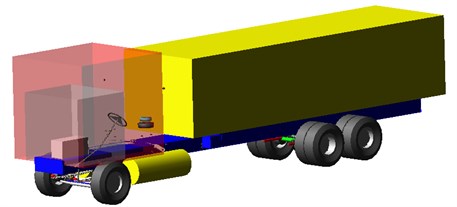
A private database shall be established before modeling to store template files established. The complete vehicle is divided into multiple different templates according to real vehicle structure of this heavy vehicle, including front suspension, tires, drive axle, plate spring, frame, steering system, rear suspension, driver’s cab, engine, etc. The multi-body dynamic model of complete vehicle generally assembled is shown in Fig. 2.
Fig. 1Flow chart of modeling of complete vehicle system
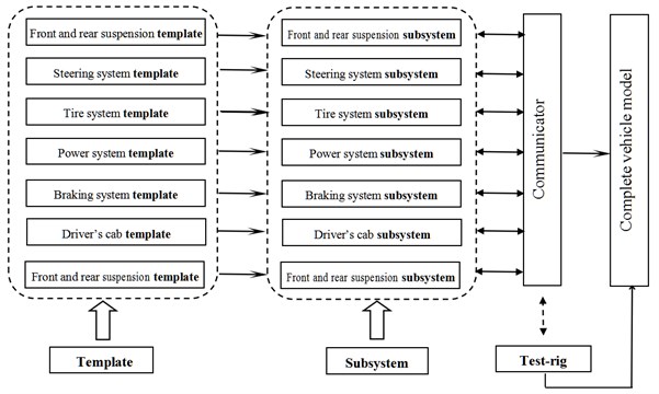
Fig. 2Multi-body dynamic model of heavy vehicle
2.2. Validating of complete vehicle model based on experimental data
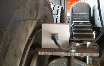
The signal acquisition systems of vehicle test mainly include three-direction speed sensor, charge amplifier, signal acquisition instrument and computer. TSC-D3 speed sensor produced by Chengdu Zhongke Measurement and Control Co., Ltd. is adopted with frequency range of 1-500 Hz. Signal acquisition instrument is adopted to convert piezoelectric signal to digital signal. INV360DF acquisition, handling and analysis instrument produced by China Orient Institute of Noise & Vibration is adopted. The experiment site and acquisition instrument adopted in the experiment are shown in Figs. 3-6 represent site layout diagrams of speed sensor in measuring points of steering front axle head, balanced suspension middle axle head and rear axle head respectively.
Fig. 3Experiment and acquisition site
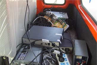
Fig. 4Measuring point of front axle head
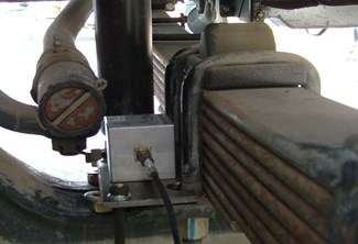
Fig. 5Measuring point of middle axle head
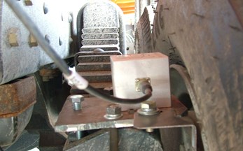
Fig. 6Measuring point of rear axle head
The simulated graphs become close to experimental graphs through debugging of characteristic parameters of virtual sample vehicle including suspension rigidity, damping and pillowslip so as to check the accuracy of complete vehicle model established. Only a part of comparison results is selected here. Under the testing conditions of full load of vehicle, B-class random road and speed of 40 km/h, lateral and vertical velocity in time domain and frequency domain in each axle are compared with simulated data and the results are shown in Table 1.
Table 1Comparison between experiment and simulation
Measuring position | Maximum velocity (mm·s-1) | Dominant frequency value (Hz) | ||
Simulation | Experiment | Simulation | Experiment | |
Lateral direction of left front axle | 36.33 | 36.41 | 0.98 | 0.98 |
Vertical direction of left front axle | 102.32 | 98.67 | 2.51 | 2.51 |
Lateral direction of left middle axle | 41.58 | 42.37 | 0.987 | 1.241 |
Vertical direction of left middle axle | 110.72 | 91.87 | 6.87 | 2.53 |
Lateral direction of left rear wheel | 38.69 | 48.66 | 10.78 | 12.53 |
Vertical direction of left rear wheel | 89.61 | 86.42 | 13.71 | 10.47 |
We can see from Table 1 that the experimental and simulated time domains and frequency domains have same trends under same velocity and road conditions, while the time domain and frequency value of simulated maximum velocity are very tiny. Take lateral direction of left front axle as an example. The simulated maximum speed is 36.33 mm/s. At this point, the frequency value is 0.98. The experiment results indicate that the maximum speed of vehicle at lateral direction of left front wheel is 36.41 mm/s and the frequency value is 0.98 at this point.
3. Construction of 3D S-curve and downhill road model
There are two methods establishing a 3D road in ADAMS/Car, namely, 3D equivalent volume method and 3D spline method. The principle of 3D equivalent volume road divides a road into a series of triangular planes for analysis as shown in Fig. 7. The 3D road is divided into 6 nodes and then four triangular elements A, B, C and D are therefore defined. The emphasis of equivalent volume method is placed on road node coordinates and number matrix. 3D coordinates and road friction conditions of the road are compiled through Road Builder. Fig. 8 indicates the spatial distribution of class-B 3D road.
A quick method applying finite element method and ADAMS environment to establish special sections was put forward in this paper. The simulated sections are described as “Introduced section (160 m)-S-shaped curve (1100 m)-Exit section (160 m)-Different downhill sections”. The curve radiuses S-shaped circles are 500 m and 528 m with azimuth angles of 43.855° and 45.626° respectively. The specific generation steps of 3D road system are shown as follows:
1) Draw road linearity in CAD and output it with format of .dxf as shown in Fig. 9;
2) Import .dxf file to ABAQUS to generate assembly body and divide grids as shown in Fig. 10;
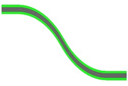
3) Run Job to generate .inp file, draw three-direction coordinates of center line, import them to Excel and edit a model same as format of road point. Directly import to ADAMS. At this point, S-curve and downhill section road are already preliminarily formed as shown in Fig. 11;
4) Open Obstacle option in road editor and set up relevant parameters to obtain desired road surface shape and road roughness.
To this end, S-curve and downhill road are already constructed. At this point, event editor and drive control file can be edited to establish a 3D road system with different slopes and different road adhesion coefficient.
Fig. 73 D equivalent volume road
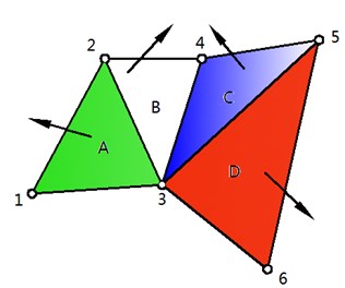
Fig. 83 D Random Road (Class-B)
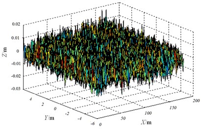
Fig. 9CAD chart of curve and downhill
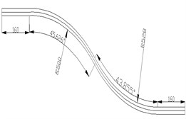
Fig. 10Division grids of curve and downhill
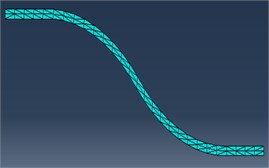
Fig. 113D road model
4. Establishment of 2D LuGre dynamical tire model
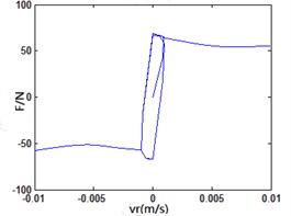
The accurate description of characteristics of contact between tire and road has an important influence on vehicle driving performance (ride comfort and handling stability) and service performance and durability of road structure. Therefore, it is very important to establish a tire physical mechanic model “communicating” with the coupling between vehicle and road. The contact between vehicle tire and road is amidst a nonlinear and non-steady dynamical acting process. Therefore, it is very necessary to apply LuGre model to the vehicle modeling, which reflects the dynamical friction contact characteristics of transient variation between tire and road. LuGre dynamical friction model is modeled according to the idea of bristle model to better accurately describe steady and dynamical characteristics during contact between tire-ground friction. LuGre model is described using differential equation of first order, including Coulomb friction, viscous friction, pre-sliding, Stribeck effect (as shown in Fig. 12), variable static friction force, friction hysteresis and steady oscillation ring, rigidity coefficient of bristle; etc., where refers to maximum static friction, refers to coulomb friction, refers to Stribeck speed, refers to relative sliding speed between friction contact surfaces. Besides compact and concise expression, the friction model can better reflect the true friction phenomenon compared with before (as shown in Fig. 13), where refers to vertical load, refers to friction force, refers to tire rotation speed, refers to tire straight-line speed.
The friction force in LuGre tire dynamical friction model is represented as average elastic deformation of bristle, please refer to Eqs. (1-3):
where, refers to rigidity coefficient of bristle; refers to microcosmic damping coefficient of bristle; refers to relative viscous damping coefficient of bristle; refers to average elastic deformation of bristle; refers to relative sliding speed between friction contact surfaces; refers to forward sliding function; refers to friction; refers to coefficient of Coulomb friction; refers to static friction coefficient; refers to Stribeck speed which is 5 m/s in the context; 1/3 refers to Stribeck index, indicating characteristic of steady friction. [0.5, 2] under general circumstances and it is determined as 0.5 in the context.
Fig. 12Stribeck effect of LuGre tire friction force
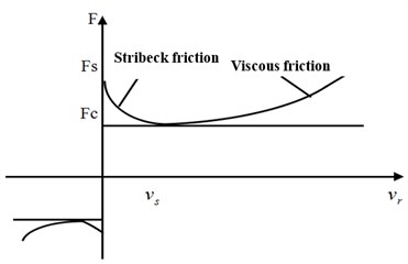
Fig. 13Contact deformation of LuGre tire model
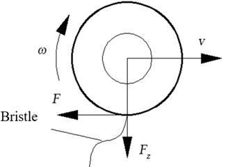
Fig. 14Friction characteristic curve upon different frequencies
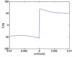
a) 0.01 Hz
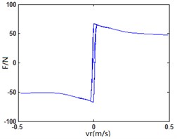
b) 0.1 Hz
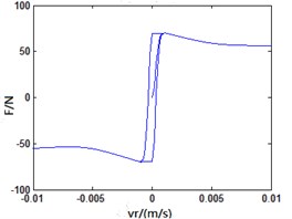
c) 1 Hz
d) 10 Hz
LuGre friction model is established in Matlab/Simulink. The sinusoidal variation of v under different frequencies is used as input to analyze the changing rules of friction force indicated in Fig. 12. When the frequency of is not big, LuGre friction model is similar to classic steady-state model; when the frequency of increases, the model indicates an obvious “hysteresis” phenomenon. Besides, the bigger the frequency and the more obvious “hysteresis” phenomenon will become. It indicates that LuGre friction model can well reflect transient response and “hysteresis” characteristic of friction between vehicle tire and road as shown in Fig. 14.
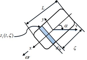
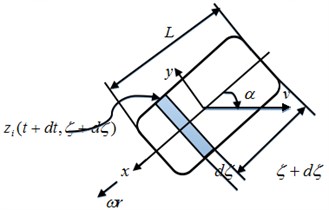
LuGre tire model is classified into four types, namely, lumped tire model, distribution tire model, an-isotropic tire model and steady-state model. When the tire is under joint condition, the unit module at moment moves along the tire rolling direction of axis and the bristle is deformed along both axis and axis under the condition that an-isotropic nature of tire is considered. It is recorded as . Then, the deformation of bristle of each unit module at moment is . See Fig. 15 for details, where is length of tire contact patch, is sideslip angle. Therefore, can be represented as Eq. (4):
Fig. 15Graphs of LuGre tire with time change
a)
b)
Represent as function involving and :
Meanwhile:
The following Eq. (7) can be obtained from Eq. (5) and Eq. (6):
When Eq. (2) is combined, the following can be obtained:
Where:
The expressions of longitudinal force , lateral force and alignment torque of tire can be obtained as follows Eq. (11) and Eq. (12):
where, refers to pressure density distribution function along the direction of contact patch of tire. When and are constant, the vehicle is under the stable driving status with established. Then, the steady-state analytical solution of can be obtained:
where:
The research indicated that the pressure distribution f tire under rolling status presented a “bell jar” shape. Aguilar-Martínez (2015) [24] provide an experimental setup for analysis of the tire-road contact area was designed and constructed. The experimental results confirmed the trapezoidal shape of the force distribution along the contact patch in the longitudinal direction.
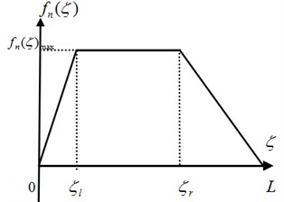
This point has been studied by Deur (2002) [25], where calculations were made to find a trapezoidal distribution of force. The longitudinal force model and lateral force model of tire were basically free from the influence of heterogeneous distribution of pressure, while alignment force model was greatly influenced by pressure distribution. Therefore, uniform pressure distribution is obtained for longitudinal force model and lateral force model in this paper, while trapezoid distribution is obtained for vertical load in the alignment force expression, shown in Fig. 16, where refers to the pressure distribution function along the direction of contact patch of tire, refers to left inflection point of trapezoid pressure distribution, refers to right inflection point of trapezoid pressure distribution, refers to the maximum value of the normal load distribution.
Fig. 16Diagram of trapezoid pressure distribution
The expression is shown as follows:
Accordingly, the expressions of longitudinal and lateral steady-state tire force and alignment torque are shown as follows:
where:
In LuGre tire model, and can be directly measured through experiment; can be calculated by formula according to parameters such as speed, wheel speed and slip angle of tire; and Stribeck index were insignificantly influenced by experimental conditions. They are determined as constants in the context. Therefore, the parameters of model to identify are , , , and where , and are static parameters, while and are dynamic parameters. The identification of static parameters can be directly fitted using experimental data under steady-state condition, while it is relatively difficult to identify dynamic parameters. Currently, there is no very mature method yet.
4.1. Construction of LuGre dynamical tire model in Simulink
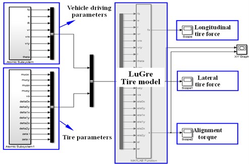
It is explained that it is very important to establish a tire physical mechanic model “communicating” with the coupling between vehicle and road. Therefore, it is very necessary to apply nonlinear LuGre model to the whole vehicle modeling, which reflects the dynamical friction contact characteristics of transient variation between tire and road. The tire model established in this paper includes two major parts, i.e. vehicle operation parameter subsystem and tire model parameter subsystem, involving 21 parameters in total. The vehicle operation parameter subsystem has 8 input parameters, namely, tire vertical load , wheel speed , wheel rolling radius , relative speed and its components along direction and direction , i.e. and , tire contact patch length and road adhesion coefficient theta. LuGre tire model parameter subsystem has 13 input parameters, namely, longitudinal and lateral Coulomb friction coefficients and , longitudinal and lateral static friction coefficients and , Stribeck speed , tire longitudinal and lateral rigidity coefficients and , tire longitudinal and lateral damping coefficients and , tire longitudinal and lateral relative viscous damping parameters and and trapezoid pressure distribution left and right inflection points and . The foregoing is used as inputs and Eq. (17) and Eq. (18) are adopted to obtain the mathematical expressions of longitudinal force , lateral force and alignment torque . The calculation of each subsystem is based on their respective input parameters. MATLAB equation code is embedded in the built-in MATLAB function module in Simulink public module library to realize the calculation of relevant longitudinal force, lateral force and alignment torque as well as output the results. The specific logic diagram of dynamical tire model is shown in Fig. 17.
Fig. 17Construction of LuGre dynamical tire model
4.2. Complete Vehicle dynamical model based on co-simulation
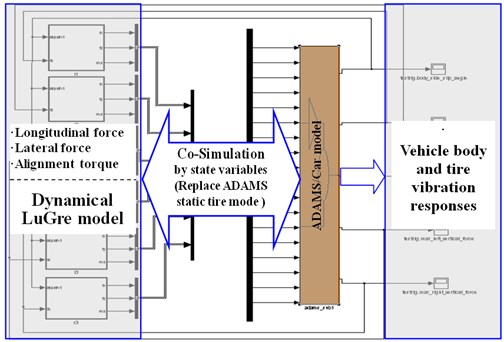
The core for realization of co-simulation interface between ADAMS/Car complete vehicle model and LuGre tire model lies in the selection of input and output parameters between the two. In the six-wheel LuGre tire model established in this paper, front and rear tire forces are marked as , , , , and . The input parameters of ADAMS/Car model include longitudinal force , lateral force and alignment torque of six wheels, while the output parameters of ADAMS/Car model include vertical load and slip angle. The principle of co-simulation between vehicle and dynamical tire model is shown in Fig. 18.
Fig. 18Co-simulation between vehicle and dynamical tire model
4.3. Checking of Tire Model Based on Co-simulation
Simulated comparison of LuGre tire model and self-fitted tire complete vehicle model is carried out to compare with longitudinal force, lateral force, vertical force and alignment torque imposed on six wheels and further verify the correctness of combination of LuGre tire model to complete vehicle model. The simulated conditions are as follows: Speed as 60 km/h; S-curve and downhill; average slope as 2 %. Due to limitation of space, only comparison diagram of each index of left front wheel is provided herein as shown in Fig. 19.
It is thus clear that the trend and amplitude of three-direction tire force and alignment torque of LuGre type model are similar to those of self-fitted Pac2002 tire model, thus verifying availability of dynamic tire established in simulated analysis of dynamics of complete vehicle.
Fig. 19Comparison diagram of dynamical load of tire
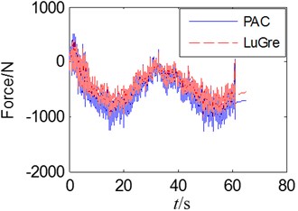
a) Longitudinal force
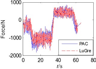
b) Latern force
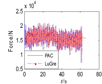
c)

d)
5. Analysis on ride comfort of vehicle in special sections
So far, the evaluation indexes and methods adopted at home and abroad on ride comfort of vehicle differ greatly especially for heavy vehicles. According to the stipulations of ISO2631-1/; 1997 (E), when the waveform peak factor of vibration signal is < 9, the root-mean-square value of weighted acceleration is adopted to evaluate the ride comfort of truck driving; when the waveform peak factor of vibration signal is > 9, the fourth root value is usually adopted to assist the evaluation of ride comfort. The relationships of root-mean-square value of weighted acceleration and weighted vibration level with people’s subjective feelings have been provided in relevant international standard.
5.1. Speed simulation for ride comfort and result analysis
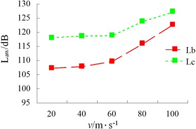
On the most common class-B and class-C random asphalt roads, the vehicle is driven on slope-free road of S-curve built at different speeds to analyze influence of different speeds on ride comfort of vehicle. The analysis results are shown in Figs. 20-23.
The following conclusions are drawn through analysis:
1) We can see from Fig. 20 and Fig. 21 that the vehicle driving speed has a relatively significant influence on ride comfort. With the increase of speed, the three-direction acceleration of driver’s cab presents a rising trend. The influence on lateral force is the most sensitive during high-speed stage; with the increase of speed, vehicle’s ride comfort becomes worse. On class-B road, when the speeds are 20 km/h, 40 km/h and 60 km/h, 0.315 and 110 dB. At this point, the driver does not feel uncomfortable. When the speed reaches 80 km/h, 0.629 and 115.838. At this point, the driver begins to feel uncomfortable. When the speed reaches 100 km/h, 1.345 and 122.576. At this point, the driver feels very uncomfortable. On class-C road, when the speed is 20 km/h, 0.805 and 118.123. The driver feels uncomfortable at this speed. When the speed is 100 km/h, 2.224 and 126.931. At this point, the driver feels extremely uncomfortable.
2) We can see from Fig. 22 and Fig. 23 that the road has an extremely big influence on ride comfort. When the speed is less than 60 km/h, the change is not significant. When the speed is greater than 60 km/h, the total weighted acceleration rises perpendicularly. The total weighted root mean square of acceleration at same speed differs greatly as well. The poorer the road and the bigger the weighted root mean square value of acceleration, the bigger the weighted vibration level and the poorer the ride comfort will become. It is thus clear that lowering of speed and improving of roughness of road surface are effective approaches to improve ride comfort. In order to improve driver’s comfort, the speed of full-load goods van shall be best controlled within 60 km/h on class-B road. On a class-C road, the driver feels uncomfortable even if the speed is only 20 km/h. Therefore, road roughness has a great influence on ride comfort of the vehicle.
Fig. 20Three-direction acceleration of driver’s cab (Class-B Road)
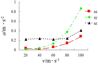
Fig. 21Three-direction acceleration of driver’s cab (Class-C Road)
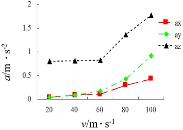
Fig. 22Total weighted acceleration of driver’s cab
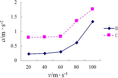
Fig. 23Total weighed vibration level of driver’s cab
5.2. Influence of different slopes on ride comfort of vehicle
As for roads with slope of 2 %-10 %, simulation of different slopes is conducted to obtain each acceleration and power spectral density of driver’s cab. The ride comfort of driver under different slopes and at each speed is shown in Table 2. In order to further analyze the reason of instability of vehicles in special sections, the different braking forces of the vehicle at speed of 40 km/h are analyzed as shown in Fig. 24.
Table 2Weighted root-mean-square value of driver’s cab. (Note: √ indicates no discomfort, while × indicates failed simulation)
Slope / % | 20 (km/h) | 40 (km/h) | 60 (km/h) | 80 (km/h) | 100 (km/h) |
2 | √ | √ | 0.29 | 0.62 | 1.61 |
3 | √ | √ | 0.26 | 0.63 | 1.74 |
4 | √ | √ | 0.26 | 0.65 | × |
5 | √ | √ | 0.31 | × | × |
6 | √ | √ | 0.41 | × | × |
7 | √ | 0.23 | × | × | × |
8 | √ | 0.24 | × | × | × |
9 | 0.21 | 0.27 | × | × | × |
10 | × | × | × | × | × |
Fig. 24Braking force under different slopes
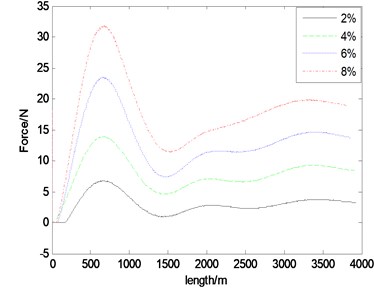
The following conclusions are drawn through comparison with above mentioned analysis:
(1) When the slope is 2 % and the speed is lower than 60 km/h, the driver does not feel uncomfortable. When the speed is 70 km/h, 0.38 m/s2. At this point, the driver feels a little uncomfortable. When the speed is 80 km/h, 0.62 m/s2. At this point, the driver is very uncomfortable. When the speed is 100 km/h, 1.60 m/s2. At this point, the driver is extremely uncomfortable. Therefore, in consideration of ride comfort of driver, the speed shall be restricted as lower than 70 km/h.
(2) When the slope is 4 % and the speed is lower than 60 km/h, the driver does not feel uncomfortable. When the speed is 70 km/h, 0.443 m/s2. At this point, the driver feels a little uncomfortable. When the speed is 80 km/h, 0.65 m/s2. At this point, the driver is very uncomfortable. When the speed is 90 km/h, 2.35 m/s2. At this point, the driver is extremely uncomfortable. When the speed is 100 km/h, simulation fails. Therefore, in consideration of ride comfort of driver, the speed shall be restricted as lower than 60 km/h and it is strictly prohibited to exceed 90 km/h.
(3) When the slope is 6 % and the speed is lower than 60 km/h, the driver does not feel uncomfortable. When the speed is 60 km/h, 0.413 m/s2. At this point, the driver feels a little uncomfortable. When the speed is 70 km/h, the brake fails to result in failure of simulation due to excessive braking force. Therefore, in consideration of ride comfort of driver, the speed shall be restricted as lower than 50 km/h and it is strictly prohibited to exceed 70 km/h.
(4) When the slope is 8 % and the speed is lower than 50 km/h, the driver does not feel uncomfortable. When the speed is 60 km/h, the brake fails to result in failure of simulation due to excessive braking force. Therefore, in consideration of ride comfort of driver, the speed shall be restricted as lower than 50 km/h and it is strictly prohibited to exceed 50 km/h.
(5) When the slope is 10 % and the speeds are 20 km/h, 30 km/h and 40 km/h, the brake fails to result in failure of simulation due to excessive braking force. Therefore, during road design, the slope shall not be too big.
It is thus clear that slope not only influences ride comfort but also causes very serious consequences if it is excessive to result in failure of braking. Therefore, big-slope road shall be avoided as much as possible. Stipulations concerning maximum road slope and speed are shown in Table 3 after consulting of stipulations set out in Detailed Rules for Design of Road Project Line (JTG-TD20-2006) [26] or Technical Standard for Road Engineering (JTG B01-2014) [27]. The simulation results reflect the relationship between maximum slope and speed in Table 4. The correctness of model and simulation results is thus further explained.
Table 3Maximum road slope
Design speed / km·h-1 | 120 | 100 | 80 | 60 | 40 | 30 | 20 |
Max slope / % | 3 | 4 | 5 | 6 | 7 | 8 | 9 |
Table 4Maximum road slope calculated based on dynamic tire
Design speed / km·h-1 | 100 | 80 | 60 | 40 | 20 |
Slope / % | 3 | 4 | 6 | 7 | 9 |
6. Simulation of driving safety in special sections
6.1. Influence of different speeds on driving safety
Simulation condition: S-curve, class-B, dry asphalt road. The results of each index of simulation of influence of speed on vehicle driving safety are shown in Figs. 25-30.
Speed has a relatively obvious influence on lateral force of each tire of vehicle. With the increase of speed, the sudden changes of tire force, alignment torque, sideslip angle and roll angle become increasingly obvious in S-curve and the tire bears increasing impact force.
Fig. 25RMS of Wheel horizontal force
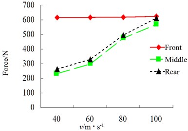
Fig. 26RMS of wheel lateral force
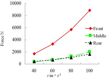
Fig. 27RMS of wheel vertical force
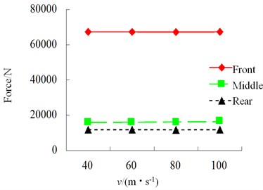
Fig. 28RMS of wheel alignment torque
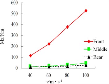
Fig. 29RMS of wheel sideslip angle
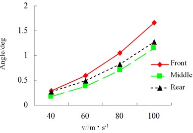
Fig. 30RMS of wheel roll angle
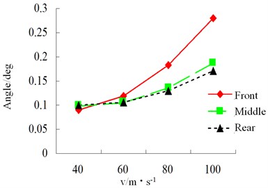
Fig. 31RMS of wheel horizontal force
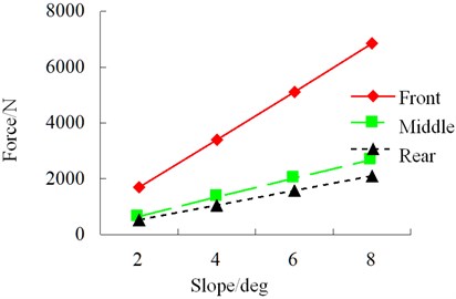
Fig. 32RMS of wheel lateral force
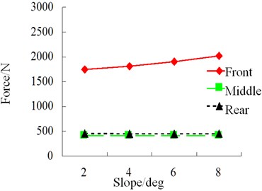
Fig. 33RMS of wheel vertical force
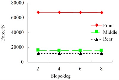
Fig. 34RMS of wheel alignment torque
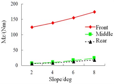
Fig. 35RMS of wheel sideslip angle
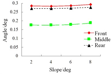
Fig. 36RMS of wheel roll angle
6.2. Influence of slope on driving safety
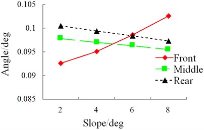
Simulation condition: S-curve, class-B random road, speed 40 km/h. The results of each index of simulation of influence of slope on vehicle driving safety are shown in Figs. 31-36.
During driving, the road slope has a relatively obvious influence on horizontal force and roll angle of the vehicle. However, in an S-curve, sudden changes still occur to lateral force, alignment torque and sideslip angle. Therefore, road scope has a great influence on vehicle safety.
7. Conclusions
Vehicle safe driving is closely related to tire-road adhesion status. Upon sudden acceleration or braking of the vehicle, the contact between vehicle tires and road is under a nonlinear and non-steady dynamical action process. However, the contact with road is always simplified as point contact and the static friction model of tire is adopted, which has ignored physical property of friction and dynamic process of establishment of friction force. It did not consider the dynamical characteristics of contact between tire and road when the vehicle passes through a curved section, which will result in the failure to reflect some important dynamical responses. Therefore, research on Stribeck dynamical friction contact model capable of truly reflecting the transient variation between tire and road was launched in this paper. The finite element method was applied to put forward a new 3D complicated road model construction method to construct roads of different classes and long-downhill paths of different S-curves. Thus, the complete research system of “Checking of virtual vehicle – Introduction of dynamical tire – Construction of vehicle-tire-ultimate road coupling system – Simulation analysis of ride comfort and safety” is proposed, so as to provide theoretical basis for road alignment design and reasonable driving speed. As a result, the following conclusions are drawn:
1) Influence of different speeds on ride comfort. When the vehicle is full-load and driven on a random class-B road involving long-downhill slope of S-curve, the speed shall be lower than 60 km/h. When the vehicle is driven on a class-C road, the driver feels uncomfortable even if the speed is only 20 km/h. Therefore, the curve road has a relatively significant influence on ride comfort of the vehicle.
2) Influence of different slopes on ride comfort. Road slope not only influences ride comfort but also causes very serious consequences if it is excessive to result in failure of braking. Therefore, big-slope road shall be avoided as much as possible.
3) Influence of different speeds and slopes on vehicle safety. With changes of vehicle driving speed, road class and change of slope, each index changes significantly especially during the S-curve where each index changes suddenly.
The transient responses of longitudinal sliding and lateral sliding of vehicle under complicated line conditions are simulated in this paper. In the next step, joint control objectives including vehicle’s active safety, handling stability and ride comfort can be realized through formulation of vehicle active steering, wheel sliding rate and semi-active suspension control strategies.
References
-
Greenwood J. A., Williamson J. B. P. Contact of nominally flat surfaces. Proceedings of the Royal Society of London, Series A, Mathematical and Physical Sciences, Vol. 295, Issue 1442, 1966, p. 300-319.
-
Gal Le A., Guy L., Orang G., et al. Modelling of sliding friction for carbon black and silica filled elastomers on road tracks. Wear, Vol. 264, Issues 7-8, 2008, p. 606-615.
-
Carbone G. A slightly corrected Greenwood and Williamson model predicts asymptotic linearity between contact area and load. Journal of the Mechanics and Physics of Solids, Vol. 57, Issue 7, 2009, p. 1093-1102.
-
Heinrich G., Klüppel M. Rubber friction, tread deformation and tire traction. Wear, Vol. 265, Issues 7-8, 2008, p. 1052-1060.
-
Wei Y. T., Shen X. L. Theory and method of tire rolling kinematics and prediction of tire forces and moments. Journal of Mechanical Engineering, Vol. 48, Issue 15, 2012, p. 65-74.
-
Xu H. G., Ma B., Xu Y., et al. Analysis of the vehicle braking stability considering the tire and pavement features. Journal of Harbin Engineering University, Vol. 34, Issue 10, 2013, p. 1287-1293.
-
Pacejka H. B. Tyre and Vehicle Dynamics. Butterworth-Heinemann, Oxford, 2006.
-
Svendenius J., Wittenmark B. Review of Wheel Modeling and Friction Estimation. Technical Report, Department of Automatic Control, Lund Institute of Technology, 2003.
-
Barahanov N., Ortega R. Necessary and sufficient conditions for passivity of the LuGre friction model. IEEE Transactions on Automatic Control, Vol. 45, Issue 4, 2000, p. 830-832.
-
Hensen R. H. A., Molengraft M. J. G. V. D., Steinbuch M. Friction induced hunting limit cycles: A comparison between the LuGre and switch friction model. Automatica, Vol. 39, Issue 12, 2003, p. 2131-2137.
-
Freidovich L., Robertsson A., Shiriaev A., et al. LuGre-Model-Based friction compensation. IEEE Transactions on Control Systems Technology, Vol. 18, Issue 1, 2010, p. 194-200.
-
Deura J., Asgari J., Hrovat D. A 3D Brush-type dynamic tire friction model. Vehicle System Dynamics, Vol. 42, Issue 3, 2004, p. 33-173.
-
Zuo S. G., Su H., Wang J. R. Simulation of self-excited vibration of a rolling tire and its influencing factors analysis. Journal of Vibration and Shock, Vol. 31, Issue 4, 2010, p. 18-24.
-
Hashemi E., Kasaiezadeh A., Khosravani S., et al. Estimation of longitudinal speed robust to road conditions for ground vehicles. Vehicle System Dynamic, Vol. 54, Issue 8, 2006, p. 1120-1146.
-
Yamashita H., Matsutani Y., Sugiyama H. Longitudinal tire dynamics model for transient braking analysis: ANCF-LuGre tire model. Journal of Computational and Nonlinear Dynamics, Vol. 10, Issue 3, 2015, p. 031003.
-
Xu J., Peng Q. Y., Shao Y. M. Mechanism analysis of vehicle accident on surface gathered water in straight section China Journal of Highway and Transport, Vol. 22, Issue 1, 2009, p. 97-103.
-
Xu J., Peng Q. Y., Shao Y. M. Effect of changing cross-section dimension of speed bumps on impact applied to pavement and vehicles. ASCE Proceedings of ICTE, 2007.
-
You K. S., Sun L., Gu W. J. Risk analysis-based identification of road hazard locations using vehicle dynamic simulation. Journal of Southeast University (Nature Science Edition), Vol. 42, Issue 1, 2012, p. 150-155.
-
Ding H., Yang Y., Chen L. Q., et al. Vibration of vehicle-pavement coupled system based on a Timoshenko beam on a nonlinear foundation. Journal of Sound and Vibration, Vol. 333, Issue 24, 2014, p. 6623-6636.
-
Guo K. H. Vehicle Handling Dynamics Theory. Jiangsu Science and Technology Press, Nanjing, 2011.
-
Yang S. P., Lu Y. J., Li S. H. An overview on vehicle dynamics. International Journal of Dynamics and Control, Vol. 1, Issue 4, 2013, p. 385-395.
-
Lu Y. J., Yang S. P., Li S. H., et al. Numerical and experimental investigation on stochastic dynamic load of a heavy duty vehicle. Applied Mathematical Modelling, Vol. 34, Issue 10, 2010, p. 2698-2710.
-
Kutluay E., Winner H. Validation of vehicle dynamics simulation models – a review. Vehicle System Dynamics, Vol. 52, Issue 2, 2014, p. 186-200.
-
Aguilar-Martíneza J., Alvarez-Icazab L. Analysis of tire-road contact area in a control oriented test bed for dynamic friction models. Journal of Applied Research and Technology, Vol. 13, Issue 4, 2015, p. 461-471.
-
Deur J., Asgari J., Hrovat D. Dynamic tire friction models for combined longitudinal and lateral vehicle motion. Proceedings of the ASME-IMECE World Conference, New York, USA, 2001.
-
Design Specification for Highway Alignment. JTGD20-2006, Ministry of Transportation of the People’s Republic of China, China Communications Press, Beijing, 2006.
-
Technical Standard of Highway Engineering. JTG B01-2014, Ministry of Transportation of the People’s Republic of China, China Communications Press, Beijing, 2014.
Cited by
About this article

This work was supported by National Natural Science Foundation of China (Grant Nos. 11572207, 11472180, 11302138) and Natural Science Foundation of Hebei Province (Grant No. A2016210103).
