Abstract
The article discusses the mesh creation techniques for models of discs of axial-flow microturbines. A universal method of optimization of such devices, in terms of their strength improvement, has been proposed. The research focused on microturbines that can operate in combination with ORC systems, especially the ones whose discs have many structural components such as pins or chamfers. Calculations were done using the commercial software ANSYS Workbench. Both tetrahedral and hexahedral grids were used in the analysed models. The calculation time needed for the grid preparation was regarded as an important parameter. Therefore, the reference model was created using the disc slice method. The results obtained for the models that included the full complex geometry of the disc were compared with the results obtained for the reference model. The mesh size coefficient was defined. It enabled to simplify the strength optimisation method for discs of axial-flow microturbine and also made it more universal. After carrying out all analyses and computations, it was possible to develop a scheme of conduct during the optimization of the aforementioned expansion devices.
Highlights
- Two strength analysis methods that can be applied to rotor discs were compared and various ways for creating a mesh were used.
- The coefficient, dependent on the blade height of the rotor disc, was determined. This allowed for the fast creation of mesh with achieving high-accuracy results.
- A fast FEM mesh creation method for the rotor discs of axial-flow turbines has been proposed.
- A scheme of conduct was described, which uses the calculated coefficient and can be applied during strength analyses of axial-flow turbines’ discs.
- The developed method is universal and allows performing analyses of various discs of axial-flow turbines (with diameters up to 150 mm).
1. Introduction
It seems that many problems of today’s power engineering can be solved by replacing big conventional power units with distributed energy systems [1-4], which can use alternative energy sources or low-temperature heat which is readily available, contrary to the heat used in high-power power plants; for example, in the most efficient ultra-supercritical power plants [5]. An ORC (organic Rankine cycle) system is one of the technologies that have gained in popularity over recent years [6-8]. As its name suggests, it is a slightly modified Rankine cycle In an ORC system, a low-boiling fluid (instead of water) is used as a working medium [9-12]. It is important to note that the use of such a fluid means that a liquid-vapour phase change occurs at a lower temperature than the water-steam phase change - in a Rankine cycle. Working fluids that are used in ORC systems are similar to those used in refrigerating cycles. The fact that the working medium can evaporate in a low temperature enables the use of ORC systems in the domestic environment. They can operate in combination with solar collectors or biomass-fired boilers and can be used for waste heat recovery [13-16]. Moreover, during the building of new installations, their designers try to minimise CO2 emissions, which is a positive trend worth mentioning[17, 18]. In today’s power engineering, very often protection of the natural environment plays first fiddle. Therefore, ORC systems are more and more popular [19] and due to the advances in their development [20], they become cheaper. Even ten years ago, ORC systems were very expensive. Besides such technologies as CNC machining (which is standard nowadays), also 3D printing technologies can be used during manufacturing of ORC systems. 3D printing techniques continue to evolve [21], paving the way for the development of machinery of certain types.
Like the Rankine cycle, the organic Rankine cycle is used to convert thermal energy to mechanical energy. The working fluid is first evaporated and then passed through an expansion device (for example, a turbine) in which the just now mentioned conversion takes place. In organic Rankine cycles, axial-flow microturbines are usually used as expansion machines [22]. The higher the efficiency of an ORC system, the more popular it can become. Obviously, the efficiency of the entire ORC system is heavily dependent on the efficiency of its expansion device. Today’s software for engineers enables carrying out advanced flow optimizations in order to achieve the best possible power output and efficiency [23]. As a result of that, the discs of axial-flow microturbines sometimes are very complex in shape and more vulnerable to high stresses. Therefore, there is a necessity to use special materials, do accurate strength computations and carry out optimizations in terms of strength [24].
2. The statements of finite elements analysis of microturbine disc
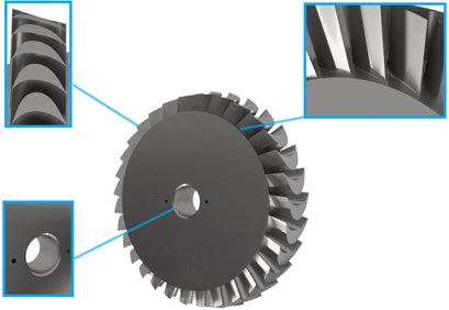
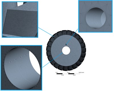
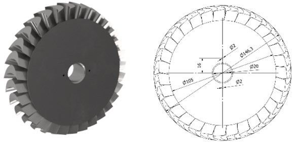
An example of a turbine disc that is complex in shape is presented in Fig. 1. Usually, the blades of a microturbine disc are not cylindrical in shape, the edge of attack and the trailing edge are not situated on the same height in each blade and the passages are non-uniformly shaped. During the optimization process, the FEM analysis (utilising various mesh creation methods) is the most commonly used tool. In commercial software, for the majority of applications meshes are created using hexahedron or tetrahedron finite elements. A hexahedron is any polyhedron with six faces. A tetrahedron, also known as a triangular pyramid, is a polyhedron composed of four triangular faces. A structured grid composed of hexahedron elements (whose six faces are in the shape of a square) is considered to be the most accurate in terms of shape mapping. However, it is usually not possible to use such a grid in modelling the discs of axial-flow microturbines because such machines have structural components such as fillet radiuses, chamfers and small holes (made, for example, for fixing certain components), which often are not symmetrical. For this reason, a mesh composed of hexahedron elements is not able to accurately map the real shape and its use either leads to obtaining wrong calculation results or the mesh creation process fails. A mesh composed of tetrahedron finite elements is the second above-mentioned type of mesh. All elements in this mesh have 4 vertices, 6 edges and are bounded by 4 triangular faces. In most cases, a tetrahedral mesh can be generated very quickly and automatically; usually, computer programs propose this mesh as a default one. Nonetheless, tetrahedral meshes are rarely used during modelling as they give less accurate results.
Two-dimensional (2D) models are used during carrying out analyses of turbine discs whose blades are not of complex shape. The results of such calculations are presented in article [25]. The researchers analysed the impact of the rotational speed on the stresses of the gas turbine’s disc exposed to high temperatures. They used the area weighted mean hoop stress method. The analyses were performed analytically and using the ANSYS environment. The research was aimed to estimate the range of rotational speeds at which the disc burst could happen. The mesh was created using finite elements in the form of plane figures with 4 vertices (PLANE182), which allowed to achieve satisfactory results.
Analyses of single blades or turbine discs of complex shape are done using 3D models. The authors of paper [26] calculated the stresses and displacements of the blade of a gas turbine with varying operating parameters (rotational speed, temperature). The blade was designed with internal passage cooling. The mesh was created using tetrahedron elements with a constant division in the whole model. There was a possibility to use hexahedron elements during modelling but calculations would have taken more time. The model was validated by comparing the obtained results with the results presented in the literature. The compatibility of both models was good.
The process of mesh creation is very time-consuming and sometimes takes even 80 % of the time of strength calculations. In some cases, the rotor disc slice method can be used in order to reduce calculation time, using a structured grid with a small number of nodes [27]. A serious disadvantage of this method is the fact that discs can have structural components (such as a pin, an inlet or a hole) which cannot be taken into account in a slice of a rotor disc. The FEM computer programs (ANSYS Workbench, in this case) artificially duplicate a slice of the disc so as to be able to analyse the whole disc. For example, adding one hole would require to carry out an analysis of the disc with many holes due to the duplication effect of the slice method.
Fig. 1An exemplary 3D model of the turbine disc; the following elements are enlarged: pinhole (in the bottom left corner), transition radius (in the upper right corner), blades with complex shapes (in the upper left corner)
Moreover, the calculation results are often needed on an ongoing basis and there is no time for time-consuming modifications of the model such as, for example, employing the rotor disc slice method [28]. For this reason, an attempt was made to create a universal mesh creation and calculation method for axial-flow microturbines’ discs with outer diameters up to 200 mm.
In the further part of this article, the results of the strength calculations obtained using models with structured and unstructured grids were compared between each other. The models were created using ANSYS software. The obtained stress, deformation and displacement values were analysed. Next, there is a discussion of the actions that needed to be taken in order to unify the calculations and mesh creation process of the discs. The next stage of research was to draw conclusions and develop a method and a scheme of conduct during making the strength calculations of subsequent discs of axial-flow turbines. The optimization of the geometry of the disc was carried out in terms of its stress because the obtained deformations are small and thus the strain is small. The change of the mesh creation method had no considerable impact on the obtained strain values.
3. Strength analysis of the turbine disc using different types of mesh
Making a comparison of the calculation results obtained after the use of a structured grid and an unstructured grid provides an excellent opportunity to launch a discussion on the application possibilities of unstructured grids. Structured grids (in this case, with hexahedron elements) are characterised by regular connectivity, better convergence and the ability to better map the curvatures compared to unstructured grids (in this case, with tetrahedron elements).
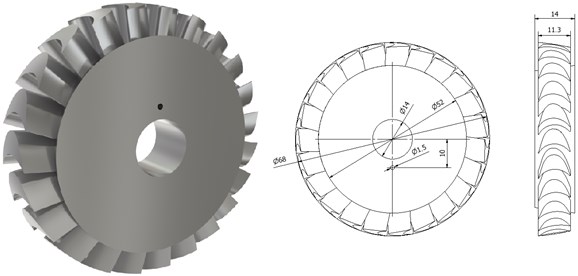
The 3D model of the turbine disc and its dimensions are shown in Fig. 2. This model was used for analysing results obtained with various types of mesh.
Fig. 23D model of the turbine disc and its dimensions
In the beginning, a structured grid (with hexahedron elements) was created as a reference grid. It was possible by using only a slice of the disc. For the calculation purposes, the disc slice was rotated several times around the rotor axis. The number of revolutions was equal to the number of blades [29]. Unfortunately, when such a method is used, it is not possible to take into account such structural components as a pin or an inlet. The highest stresses are expected to occur at the footing of the blade. Therefore, the results obtained from the models that use a structured grid and an unstructured grid can be easily compared with each other.
The model of the disc slice, for which the mesh was already created, is presented in Fig. 3. A bonded contact was set between the blade and the rotor disc. This is a special type of contact that which allows no relative displacement between two connected solid bodies. The slice was created using the Inventor software. It was a very time-consuming process. With this in mind, one can notice that the whole strength analysis takes more time.
Fig. 3Model of the disc with a diameter of 68 mm, in which the mesh is composed of hexahedron elements shown in an enlarged view (on the right side) and the element quality values are indicated by light blue arrows (on the left side)
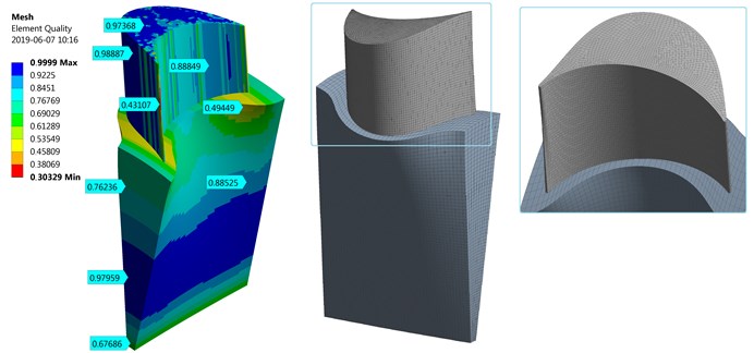
As can be seen in the figure shown above, the mesh is very accurate and systematic. Element quality values are also marked by light blue arrows. A tool available in ANSYS software, which combines most of the known methods for analysing the mesh quality (such as skewness and aspect ratio), was used to check the grid quality. The colours denote the relationship of the used finite element, where 1 (blue colour) means that all edges have the same length. In practice, elements whose coefficient of the mesh quality is lesser than 0.2 are used when strength calculations of models of complex shape are done. In the case discussed herein, the edge of attack is divided into elements of low quality because these elements are much smaller than the elements used in other parts of the model. An attempt to obtain a mesh of good quality on the edges could make the remaining finite elements to become distorted. The mesh of the disc slice contains:
– 92,240 elements;
– 400,749 nodes.
The boundary conditions, shown in Fig. 4, were as follows:
– material – PA9 (aluminium alloy);
– rotational speed – 40,000 rpm;
– movement constraint in the -axis direction;
– cylindrical support with the permissible rotary motion around the -axis.
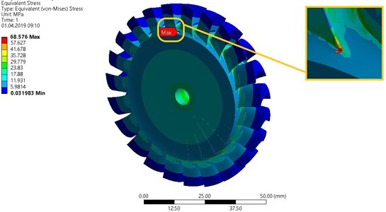
The two following figures (Fig. 5 and Fig. 6) show results obtained after using the disc slice method. The maximum displacement (about 0.0042 mm) occurs at the blade tip on the side of the edge of attack (the longer edge). The maximum and minimum deformation values are marked with light blue arrows. Furthermore, the highest stress (approx. 68 MPa) occurs at the blade footing. This place is marked with a red arrow. This may be attributable to the fact that the fillet radiuses between the surfaces of the disc and the blades were not taken into account in the models.
Fig. 4Boundary conditions that were applied to the model of the turbine disc with a diameter of 68 mm
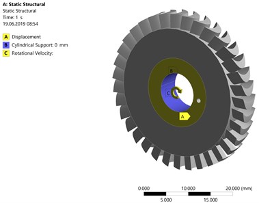
Fig. 5The elastic strain and total deformation of the turbine disc with a diameter of 68 mm
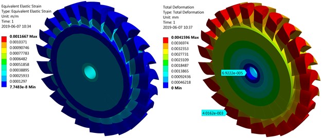
Fig. 6The equivalent von Mises stress of the turbine disc with a diameter of 68 mm, with enlarged blade footing where the stresses have the maximum value
The above results were treated as reference results and gave rise to further consideration. The next stage of the research was to create a model with a tetragonal mesh and do the calculations so as their results could differ by not more than plus or minus five percentage points from the results obtained for the model with a structured grid. The mesh in the model of the whole disc was created using tetragonal elements that have a triangle base with a shape function of the second degree (10 nodes). The global value of the length of the edges of these elements was 0.9 mm. The value of this parameter was decreased to 0.2 mm in the three parts of the model in which the highest stresses were expected, namely the hole for fixing the shaft, the hole for fixing a pin and the disc blades. Moreover, several boundary layers were added in the holes to improve the mesh quality.
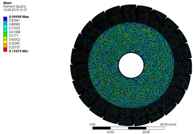
The quality of the tetragonal mesh used in the whole disc is shown in Fig. 7. One can observe that the elements are non-uniformly placed but the quality coefficient is greater or equal than the boundary value equal to 0.2 in the whole model. The quality coefficient has a value of 0.13 only for several elements situated inside the hole for fixing the shaft.
Fig. 7Quality of finite elements used in the tetragonal mesh of the model of the disc with a diameter of 68 mm
During the optimization of the mesh, the value of the coefficient was determined for turbine discs. This coefficient denotes the relationship between the maximum length of edges of the finite element used and the blade height, which is a characteristic dimension of each turbine disc. In the entire disc model, the “face size” function was used for the purposes of mesh preparation.
The element size () can be calculated using the following formula:
where – the maximum characteristic dimension of the mesh element [mm], – characteristic magnitude [mm], – mesh size coefficient [–].
The calculations were made with the same boundary conditions as in the case of calculations made for the model with the structured grid. A series of calculations was carried out for different values of the finite element size (), which is dependent upon the coefficient and the blade length. The relevant results are demonstrated in Table 1.
Table 1Results of the strength calculations of the disc with a diameter of 68 mm
No. | [–] | [mm] | [mm/mm] | [MPa] | Number of finite elements |
1 | 0.010 | 0.10 | 0.001 | 65.700 | 5.045.002 |
2 | 0.015 | 0.15 | 0.001 | 69.191 | 2.301.376 |
3 | 0.020 | 0.20 | 0.001 | 59.727 | 1.337.819 |
4 | 0.025 | 0.25 | 0.001 | 56.128 | 897.611 |
5 | 0.030 | 0.30 | 0.001 | 54.086 | 669.905 |
6 | 0.035 | 0.35 | 0.001 | 49.195 | 514.782 |
7 | 0.040 | 0.40 | 0.001 | 51.004 | 424.257 |
8 | 0.045 | 0.45 | 0.001 | 49.850 | 374.688 |
9 | 0.050 | 0.50 | 0.001 | 50.860 | 321.470 |
The highest stresses occur at the footing of the blade, somewhat reproducing the results obtained for the reference mesh composed of hexahedron elements. The differences in stress values on the blade, which were obtained using models with different finite element sizes, are large (up to 15 percentage points). However, strain and displacements do not vary significantly. In Fig. 8, there is a graph showing the maximum blade stress as a function of the mesh size coefficient.
As can be seen, the maximum stress decreases as the finite element size () increases. It stems from the complex geometry of the disc. The elements in the crucial places (in this case, the footing of the blade) distorted, which was followed by stress concentration.
The red line indicates the maximum stress obtained for the structured mesh (the reference mesh). As can be seen, similar results were obtained for the coefficient equal to 0.015. It can be assumed that the finite element size is optimal when the difference between the maximum stress obtained using the tetragonal mesh and the maximum stress obtained using the reference mesh with hexagon elements remains within the range of plus or minus five percentage points (in Fig. 5, the relevant area is marked with light red colour). For this disc, the finite element size is optimal when the coefficient is in the range of 0.01 to 0.015.
Fig. 8The blade stress vs. mesh size coefficient (results obtained for the disc with a diameter of 68 mm)
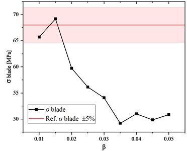
Fig. 9Calculation time and maximum usage of RAM versus β coefficient
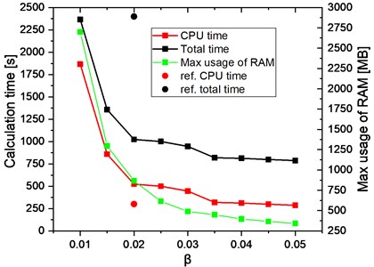
Fig. 10Model of the disc with a diameter of 68 mm, which was created using the tetragonal mesh
Calculation time is a really important parameter during the stress optimisation of the discs of axial-flow microturbines. As can be seen in Fig. 9, the calculation time (CPU time) increases significantly for low values of the coefficient. This is obviously due to the fact that the number of finite elements increases as the value of the coefficient decreases. An increase in the number of finite elements also increases the usage of RAM. However, the total time of the simulation of a single case, which is the sum of the CPU time and the preparation time of the model (i.e. discretisation, boundary conditions, the preparation of a CAD model), is a more important parameter. In the case of the proposed method where the coefficient is taken into account, the preparation time of the model is between 500 and 600 seconds and the calculation time changes according to the number of finite elements used in the mesh. For comparison purposes, the calculation times (red and black dots) obtained using the disc slice method described in the above-mentioned article are placed in the graph below. These results were treated as reference results. As can be seen in this case, the calculation time is around 50 % lower but the preparation of the model takes a lot of time.
The use of the coefficient enables to quickly determine the finite element size, without a necessity to carry out the whole optimization process. In Fig. 10, shown below, it can be seen how the tetragonal mesh looks like after the optimization. This mesh gives the same results as the mesh composed of hexagon elements.
The tetragonal mesh is very dense in the holes and on the blades but it maps the curvatures of the analysed disc extraordinarily well and gives highly accurate stress results.
4. Strength of turbine discs with different diameters
In the next stage of research, the finite element size (the tetrahedron size, in this case) was changed depending on the blade length of the turbine disc and the mesh parameters were determined for discs of various sizes. The strength calculations were also done, which made it possible to check if the mesh size coefficient had been chosen correctly.
The disc with an outer diameter of 36.2 mm (shown in Fig. 11) was analysed first. This disc is made of aluminium alloy 7075 and its maximum rotational speed is 120,000 rpm.
Fig. 11Disc whose outer diameter is 36.2 mm
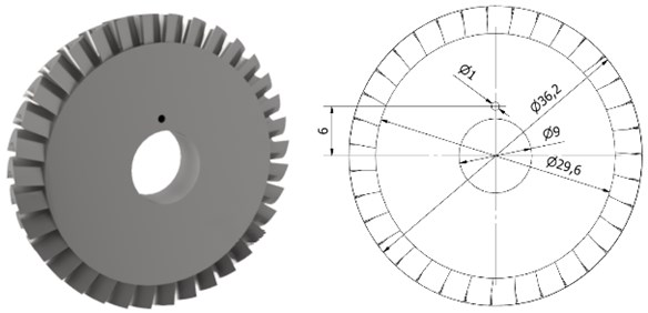
Table 2Results obtained for the disc whose outer diameter is equal to 36.2 mm
No. | [–] | [mm] | [mm/mm] | [MPa] | [MPa] | [MPa] | Number of finite elements |
1 | 0.015 | 0.45 | 0.002 | 63.884 | 157.977 | 121.598 | 5,645,034 |
2 | 0.020 | 0.20 | 0.002 | 63.871 | 157.890 | 117.637 | 3,226,861 |
3 | 0.025 | 0.25 | 0.002 | 63.881 | 157.798 | 120.743 | 2,140,528 |
4 | 0.030 | 0.30 | 0.002 | 63.927 | 157.439 | 121.055 | 1,480,987 |
5 | 0.035 | 0.35 | 0.002 | 63.908 | 158.180 | 100.365 | 1,081,951 |
6 | 0.040 | 0.40 | 0.002 | 63.885 | 158.063 | 98.817 | 849,962 |
7 | 0.045 | 0.45 | 0.002 | 63.852 | 158.092 | 106.659 | 693,784 |
8 | 0.050 | 0.50 | 0.002 | 63.867 | 157.773 | 129.660 | 592,452 |
A series of calculations was conducted, using the same boundary conditions and mesh creation methods as in the case of the disc whose diameter is 68 mm. The results obtained for the above-mentioned disc are discussed in the following part of the article. The calculations with values of the coefficient lesser than 0.015 were not made as the number of finite elements exceeded ten million.
The highest stress, about 158 MPa, occurs inside the hole for fixing a pin. However, during making a comparison between the results obtained for the disc whose outer diameter is 36.2 mm and the reference results, one should compare the results obtained on the blade because in the model created using the disc slice method it is not possible to create the hole for a pin. Although the value of the coefficient was changed, the strain was at the same level. The next figure (Fig. 12) presents a graph showing the maximum stress on the blade versus the mesh size coefficient ().
Fig. 12The blade stress vs. coefficient of the finite element size (results obtained for the disc whose outer diameter is 36.2 mm)
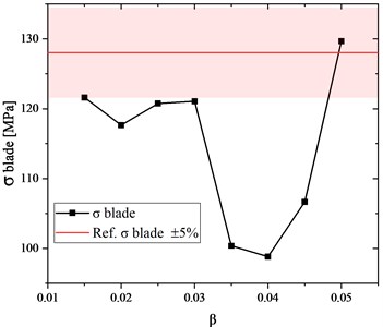
The black line demonstrates the stress versus the coefficient value while the red line indicates the stress value that was obtained using the reference mesh with hexagon elements. As can be seen, the value of the coefficient is optimal only if it remains within the range of 0.015 to 0.03. In this range, the results obtained using a structured grid and an unstructured grid differ by not more than plus or minus five percentage points.
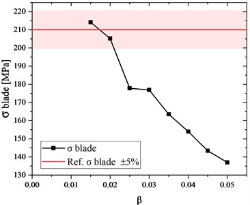
Next, calculations were done for the disc whose diameter is 146.3 mm, and whose blade height is 20 mm. The disc is made of aluminium alloy 7075 and its nominal rotational speed is 40,000 rpm. The dimensions of this disc are shown in Fig. 13.
Fig. 13Disc whose outer diameter is 146.3 mm
The obtained calculation results are listed in Table 3. The highest stresses occur in the hole for fixing the shaft. The calculation results show that the optimal value inside the hole is 0.2 mm for holes whose diameters are not greater than 35 mm. Therefore, the comparative analysis concerned the stresses on the blade.
The graph presented in Fig. 13 shows the stress on the blade versus the β coefficient. The reference value (210 MPa) is marked on the graph using a red horizontal line. This is the value that occurs on the fillet radius of the blade. The results of calculations made for the meshes whose finite element sizes were 0.015 mm and 0.02 differ only slightly from the reference value. Thus, the mesh size coefficient for this case is optimal if its value remains within the range of 0.015 to 0.02. For this turbine disc, the strain was the highest (0.0065) and was the same for different parameters of the mesh.
Table 3Results obtained for the disc whose outer diameter is equal to 146.3 mm
No. | [–] | [mm] | [mm/mm] | [MPa] | [MPa] | [MPa] | Number of finite elements |
1 | 0.015 | 0.3 | 0.0065 | 468.866 | 252.002 | 214.140 | 3.116.694 |
2 | 0.020 | 0.4 | 0.0065 | 469.329 | 260.892 | 205.136 | 2.144.713 |
3 | 0.025 | 0.5 | 0.0065 | 468.925 | 241.113 | 177.802 | 1.665.890 |
4 | 0.030 | 0.6 | 0.0065 | 470.021 | 258.988 | 176.866 | 1.438.543 |
5 | 0.035 | 0.7 | 0.0065 | 469.434 | 243.069 | 163.477 | 1.278.777 |
6 | 0.040 | 0.8 | 0.0065 | 469.647 | 258.852 | 153.994 | 1.190.666 |
7 | 0.045 | 0.9 | 0.0065 | 469.786 | 249.027 | 143.406 | 1.118.306 |
8 | 0.050 | 1 | 0.0065 | 469.754 | 258.817 | 137.016 | 1.077.457 |
Fig. 14Stress vs. coefficient of the finite element size (results obtained for the disc whose outer diameter is 146.3 mm)
5. Analysis of the obtained results
All the analysed turbine discs are or will be used as components of ORC microturbines that are developed at the Institute of Fluid-Flow Machinery in Gdańsk. The results of strength calculations will be verified as soon as the building of the installations comes to an end.
The graph, presented in Fig. 15, shows the ratio of the obtained stress to the reference stress (σ ratio) as a function of the coefficient for three turbine discs with different diameters. The axis of ordinates denotes the ratio of the obtained stress to the reference stress value (where both these values are stress values on the blade). The reference value was obtained after using the disc slice method for the mesh composed of hexahedron elements. The σ ratio value equal to 1 means that the stress values obtained using both methods are equal to each other, whereas values lesser or higher than 1 show the percentage deviation from the reference value. Looking at Fig. 15, one can analyse how the coefficient (finite element size) affects the results. The lower the value of this coefficient, the lower the difference between the obtained value and the reference value. The used method gave the best results for the largest disc (its corresponding values are marked with triangles); the curve decreases more or less linearly as the coefficient increases. For the disc whose diameter is 68 mm, when the coefficient decreases from 0.015 to 0.01 the ratio decreases as well (values marked with wheels). For the disc whose diameter is the smallest (values marked with squares), the obtained curve is irregular and decreasing the coefficient (starting from 0.03) does not cause a significant decrease in ratio. When the coefficient is equal to 0.05, higher stress values are obtained on the whole disc as compared to the disc slice method, even with the mesh of low quality and not very accurate mapping of the curvature of the edge of attack as well as of the trailing edge.
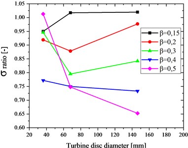
Fig. 16 demonstrates the graph showing the ratio (the ratio of the obtained stress to the reference stress) as a function of diameters of the discs discussed herein. One can notice that when the finite element size (expressed by the coefficient) is equal to 0.04, the stress values obtained for all the analysed discs significantly differ from the reference values. The differences reach 30 percentage points. For the smallest disc, the obtained stress values do not exceed the permissible percentage threshold of five per cent when the coefficient is 0.03 or 0.05. For discs of other sizes, the permissible percentage threshold was exceeded by 20 % and 35 % respectively. The best results were obtained for the models in which the coefficient was equal to 0.015 and the obtained stress values did not exceed the permissible percentage threshold for all analysed discs.
Fig. 15Ratio of the obtained stress to the reference stress vs. β (coefficient of the finite element size)
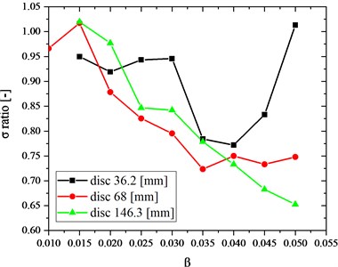
Fig. 16Ratio of the obtained stress to the reference stress vs. diameter of the turbine disc
After taking a look at the graph shown in Fig. 17, one can notice that the higher the number of finite elements, the higher the stress values in the blade. Unfortunately, when the value of the coefficient is lesser than 0.015, the number of finite elements is very large (over 10 million). One can also notice that when the number of finite elements is greater than 2 million, the improvement in the quality of stress results is not so big as for a smaller number of finite elements. The stress results of the disc of the highest diameter (i.e. the results marked with triangles) are heavily dependent on the number of finite elements.
The above-mentioned dependency is seen most clearly in Fig. 18 that presents the coefficient versus the number of finite elements. For all discs, when the coefficient is 0.05 the number of finite elements is in the range from 0.5 million to 1.5 million. Decreasing this coefficient (to some extent) does not cause a significant increase in the number of elements. For the coefficient values that are lesser than 0.03, the number of elements considerably increases, which is also reflected in changes in the stress value.
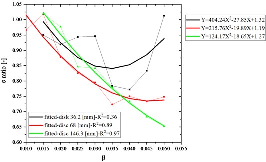
A polynomial function of the second degree was created for each curve shown in Fig. 15. The polynomials and their corresponding curves are demonstrated in Fig. 18, on the right-hand side and left-hand side, respectively. The curves, marked with bold lines in the legend of Fig. 18, are fitted to the results obtained for each disc (the coefficient of determination is denoted by ). These curves are parabolas. The parabola corresponding to the smallest disc (whose results are marked with squares) is fitted in the slightest degree. However, the greater the diameter of the disc, the more fitted the curves. It may mean that the proposed method will work better for bigger discs. What is more, after taking a closer look at the parabolas, it can be noticed that in the case of the smallest disc the analysed finite element size range was too broad. The coefficient value can be easily calculated using the equations worked out for each disc. The dependencies presented herein will serve as a basis for further work on the universal mesh creation method for the discs of axial-flow turbines.
Fig. 17Ratio of the obtained stress to the reference stress vs. number of finite elements
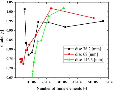
Fig. 18β (coefficient of the finite element size) vs. number of finite elements
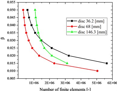
Fig. 19Ratio of the obtained stress to the reference stress vs. β (coefficient of the finite element size)
6. The proposed mesh type for the strength calculations of the turbine disc
Quite often, after creating the disc geometry, independently whether additional software was used, one can notice certain unnecessary elements (such as, for example, lines). They must be deleted. Furthermore, care needs to be taken to ensure that all elements of the disc (surfaces) are uniform, with no discontinuities since it could disturb the calculation process. However, it is not uncommon that edges of attack or trailing edges are not perfect in this respect. In some cases, the program is not able to prepare the mesh of an element, hence calculations cannot commence. First of all, the disc should be divided into the following parts (as shown in Fig. 20):
a) blades,
b) hole for fixing a pin,
c) hole for fixing the shaft,
d) disc.
The mesh should be prepared according to the hints given in Table 4. As can be seen, this process is not complex. If the disc does not have a hole for fixing a pin or a hole for fixing the shaft, there is no need to perform actions associated with one or both of these holes. When boundary conditions are laid down for axial discs, in majority of cases, the “fixed support” function is used with a chosen plane that includes a hole for fixing the shaft. However, this approach does not reflect the actual attachment method. In order to model the disc as well as possible, the “cylindrical support” function should be applied to the hole for fixing the shaft and to the disc hub (with enabling the free axial movement) as well as the “displacement” function should be applied to the place for fixing a pin (with a constraint imposed for the -axis). The next stage is related to the rotational speed or the pressure distribution on the blades, which results from the working medium flow. The parameters of the analysis are set according to the carried out analysis.
Fig. 20The turbine disc scheme on which the following parts are marked: blades (a), hole for fixing a pin (b), hole for fixing the shaft (c), disc (d)
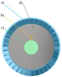
Table 4The mesh preparation procedure for the strength calculations of the turbine disc
Part denotation | Part description | Operation | Set value |
a) | Blades | Mesh densification using the “face sizing” function | Coefficient of the finite element size (0.015) |
b) | Hole for fixing a pin | Mesh densification using the “face sizing” function | From 0.1 mm to 0.2 mm |
Adding the boundary layer using the “inflation” function | Max number of layers is in the range of 4 to 7 | ||
c) | Hole for fixing the shaft | Mesh densification using the “face sizing” function | 0.2 mm |
Adding the boundary layer using the “inflation” function | Max number of layers is in the range of 4 to 7 | ||
d) | Disc | Mesh densification using the “body sizing” function | Value, for example 0.9 mm |
7. Conclusions
When doing strength calculations of turbine discs, their 3D models can be composed of tetrahedron finite elements. The greater the number of finite elements is, the higher the accuracy of calculations will be. The turbine disc model has to include a very high number of finite elements (over 2 million) in order to be able to precisely map the irregular shapes of blades. By using the coefficient it is possible to quite easily prepare the meshes for axial-flow turbines’ discs with various diameters.
The analysed parameter was the stress in the place where the blade is joined to the turbine disc. In this case, the strain of the discs was only partially dependent on the mesh quality. The designed discs are very rigid, thus the displacements of the blade tip are very low. It could change after taking into account the operating temperature of the discs, and this will be the topic of future work.
The coefficient of the finite element size, which is selected according to the height of the blades of the turbine disc, works very well in strength calculations of the discs of axial-flow turbines. In the presented analyses, the best results were obtained when the coefficient was equal to 0.015. The same conclusion was drawn after solving the polynomial equation of degree 2, which was created based on the trend line representing the results of the performed series of calculations. The use of the coefficient considerably increases the mesh preparation time and the number of finite elements; however, the total time of the analysis is much shorter in comparison with the classic approach. The diminishing of the value of coefficient caused that the number of finite elements exceeded 10 million but the obtained solution was not always more accurate.
In future, a far greater number of discs (with different diameters) will be needed to verify the proposed method. Thermal stresses will be taken into account in the model. Moreover, the chosen discs will be put to tensile tests and then the results of these tests will be compared with the results obtained from numerical models.
References
-
Fonseca J. D., Camargo M., Commenge J. M., Falk L., Gil I. D. Trends in design of distributed energy systems using hydrogen as energy vector: A systematic literature review. International Journal of Hydrogen Energy, Vol. 44, Issue 19, 2019, p. 9486-9504.
-
Garcia-Saez I., Méndez J., Ortiz C., Loncar D., Becerra J. A., Chacartegui R. Energy and economic assessment of solar Organic Rankine Cycle for combined heat and power generation in residential applications. Renewable Energy, Vol. 140, 2019, p. 461-476.
-
Modi A., Bühler F., Andreasen J. G., Haglind F. A review of solar energy based heat and power generation systems. Renewable and Sustainable Energy Reviews, Vol. 67, 2017, p. 1047-1064.
-
Renewable Energy Policy Network for the 21st Century, Renewables 2015 Global Status Report, 2015.
-
Rogalev N., Golodnitskiy A., Tumanovskiy A., Rogalev A. A survey of state-of-the-art development of coal-fired steam turbine power plant based on advanced ultrasupercritical steam technology. Contemporary Engineering Sciences, Vol. 7, Issue 2014, 34, p. 1807-1825.
-
Colonna P., Casati E., Trapp C., Mathijssen T., Larjola J., Turunen Saaresti T., Uusitalo A. Organic Rankine cycle power systems: from the concept to current technology, applications, and an outlook to the future. Journal of Engineering for Gas Turbines and Power, Vol. 137, Issue 10, 2015, p. 100801.
-
Dual A., In E. Experimental study on the organic Rankine cycle power system. Proceedings of ASME Turbo Expo, 2014.
-
Dickes R., Dumont O., Legros A., Quoilin S., Lemort V. Analysis and comparison of different modeling approaches for the simulation of a micro-scale organic Rankine cycle power plant. Proceedings of the 3rd International Seminar on ORC Power Systems, 2015.
-
Yamada N., Mohamad M. N. A., Kien T. T. Study on thermal efficiency of low- to medium-temperature organic Rankine cycles using HFO-1234yf. Renewable Energy, Vol. 41, 2012, p. 368-375.
-
Invernizzi C. M., Iora P., Preßinger M., Manzolini G. HFOs as substitute for R-134a as working fluids in ORC power plants: A thermodynamic assessment and thermal stability analysis. Applied Thermal Engineering, Vol. 103, Issue 25, 2016, p. 790-797.
-
Moroz L., Kuo C.-R., Guriev O., Li Y.-C., Frolov B. Axial turbine flow path design for an organic rankine cycle using R-245fa. ASME Turbo Expo: Turbine Technical Conference and Exposition, 2013.
-
Micheli D., Pinamonti P., Reini M., Taccani R. Performance analysis and working fluid optimization of a cogenerative organic rankine cycle plant. Journal of Energy Resources Technology, Vol. 135, Issue 2, 2013, p. 021601.
-
Sellers C., Hawkins L. Development of a 350kW marine organic rankine power module for ship waste steam. ASME Turbo Expo 2017: Turbomachinery Technical Conference and Exposition, 2017.
-
Cogswell F. J., Gerlach D. W., Wagner T. C., Mulugeta J. Design of an organic rankine cycle for waste heat recovery from a portable diesel generator. ASME International Mechanical Engineering Congress and Exposition, 2011.
-
Han T., Huang K., Hung T.-C., Lin C.-R. Performance analysis for an organic rankine cycle using engine exhaust gas as heat source. Inaugural US-EU-China Thermophysics Conference-Renewable Energy 2009.
-
Klonowicz P., Witanowski Ł., Jȩdrzejewski Ł., Suchocki T., Lampart P. A turbine based domestic micro ORC system. Energy Procedia, Vol. 129, 2017, p. 923-930.
-
AlZahrani A. A., Dincer I. Comparative energy and exergy studies of combined CO2 Brayton-organic Rankine cycle integrated with solar tower plant. International Journal of Exergy, Vol. 26, Issue 1/2, 2018, p. 21.
-
Sachdeva J., Singh O. Thermodynamic analysis of solar powered triple combined Brayton, Rankine and organic Rankine cycle for carbon free power. Renewable Energy, Vol. 139, 2019, p. 765-780.
-
Żywica G., Drewczyński M., Kiciński J., Rządkowski R. Computational modal and strength analysis of the steam microturbine with fluid-film bearings. Journal of Vibrational Engineering and Technologies, Vol. 2, Issue 6, 2014, p. 543-549.
-
Kaczmarczyk T. Z., Zywica G., Ihnatowicz E. Experimental study of a low temperature micro-scale organic Rankine cycle system with the multi-stage radial-flow turbine for domestic applications. Energy Conversion and Management, Vol. 199, 2019, p. 111941.
-
Zywica G., Kaczmarczyk T., Ihnatowicz E., Baginski P. L., Andrearczyk A. Design and manufacturing of micro-turbomachinery components with application of heat resistant plastics. Mechanics and Mechanical Engineering, Vol. 22, Issue 2, 2018, p. 649-660.
-
Maharaj C., Morris A., Dear J. P. Modelling of creep in Inconel 706 turbine disc fir-tree. Materials Science and Engineering A, Vol. 558, 2012, p. 412-421.
-
Fu L., Shi Y., Deng Q., Li H., Feng Z. Integrated optimization design for a radial turbine wheel of a 100 kw-class microturbine. Journal of Engineering for Gas Turbines and Power, Vol. 134, Issue 1, 2011, p. 012301.
-
Ma Y., Zhang Y., Zhang H., Xue C. Residual stress analysis of the multi-stage forging process of a nickel-based superalloy turbine disc. Proceedings of the Institution of Mechanical Engineers, Part G: Journal of Aerospace Engineering, Vol. 227, Issue 2, 2013, p. 213-225.
-
Kumar R., Ranjan V., Kumar B., Ghoshal S. K. Finite element modelling and analysis of the burst margin of a gas turbine disc using an area weighted mean hoop stress method. Engineering Failure Analysis, Vol. 90, 2018, p. 425-433.
-
Tong F., Gou W., Li L., Gao W., Feng Yue Z. Thermomechanical stress analysis for gas turbine blade with cooling structures. Multidiscipline Modeling in Materials and Structures, Vol. 14, Issue 4, 2018, p. 722-734.
-
Meguid S. A., Kanth P. S., Czekanski A. Finite element analysis of fir-tree region in turbine discs. Finite Elements in Analysis and Design, Vol. 35, Issue 4, 2000, p. 305-317.
-
Zywica G., Kiciński J. The influence of selected design and operating parameters on the dynamics of the steam micro-turbine. Open Engineering, Vol. 5, Issue 1, 2015, p. 385-398.
-
Li J., Lie S. T., Cen Z. Numerical analysis of dynamic behavior of stream turbine blade group. Finite Elements in Analysis and Design, Vol. 35, Issue 4, 2000, p. 337-348.
Cited by
About this article

