Implementation of lookup tables for different optimization strategies of semi-active car suspension system

Čerškus, Aurimas; Šešok, Nikolaj; Bučinskas, Vytautas

doi:10.21595/jve.2025.24689

Journal of Vibroengineering

Browse Journal

Submit article

Published: 05 April 2025

Check for updates

Implementation of lookup tables for different optimization strategies of semi-active car suspension system

Aurimas Čerškus¹

Nikolaj Šešok²

Vytautas Bučinskas³

^{1, 2, 3}Department of Mechatronics, Robotics and Digital Manufacturing, Vilnius Gediminas Technical University, Vilnius, Lithuania

Corresponding Author:

Vytautas Bučinskas

Cite the article Download PDF

Downloads 39

Abstract

Road irregularities and various vehicle loads influence comfort and safety levels. Owing to these changes, the driver cannot quickly and easily find the best driving parameters. Control of damping in a semi-active suspension adjusts the damping process in the vehicle to minimize the acceleration of the crew. This ensures comfort for them, influencing the level of fatigue of the driver and safe driving. A theoretical analysis was implemented using a mathematical full-car model in Simulink/MATLAB. We performed a simulation of a vehicle with all passengers passing various artificially generated road profiles at different velocities. We optimized the damping coefficient for the maximum comfort level using one, two, or four damping values, implementing different optimization strategies. The obtained research results were finalized by the conclusions.

Implementation of lookup tables for different optimization strategies of semi-active car suspension system

Highlights

Semi-active vehicle suspension, whcih can improve comfort with minimum energu losses
Novel approach for suspension modelling
Obtained semi-active suspension efficiency
Obtained limitations on damping effciency

1. Introduction

One of the key systems in a vehicle is the suspension, which helps to maintain uninterrupted and good touch of the tires with the road and assures driving safety and ride comfort irrespective of the quality of the road surface or weather conditions [1]-[3]. The suspension can be passive, fully active, or semi-active. Typically, passive suspension systems have limited isolation or motion control. The crew is best isolated from low-frequency vibrations when damping is high. However, high damping reduces high-frequency absorption. Conversely, when the damping is low, the damper offers sufficient high-frequency absorption and poor low-frequency isolation. D. Karnopp [4] stated that for ride comfort, the suspension should isolate the body from high-frequency road inputs. However, at lower frequencies, the body and wheel should closely follow the vertical input from the road. This is related to vehicle handling. Thus, the increased damping in the suspension system deteriorates comfort but improves safety. The intuitive relationship between comfort and safety is discrepant [1], [5], [6], and it is not viable to improve both at the same time. Meanwhile, the authors [7], [8] showed that the dependence of modified comfort and safety indicators on some damping ranges of damping increases and decreases consistently. Another possible solution to this compromise is the semi-active hydropneumatic spring-damper system proposed by P.S. Els et al. [1], in the form of a four-state system, or an active suspension system, or improving driver comfort by optimizing the seat [9]. Various systems have been discussed in references [3], [5], [10]-[12], and their strengths, weaknesses, relative performance, and equipment requirements have been identified. Active suspension systems can improve the performance of suspension systems at wide frequencies compared to passive suspension systems [13]. A semi-active suspension system combines the advantages of other types of suspensions. It can smoothly change damping, be effective nearly as effective as a fully active suspension [14], and is preferred due to its inherent characteristics such as low energy consumption, especially in vehicles where available power is limited. Semi-active suspensions have attracted considerable attention because their controllable parameters can be adjusted in real-time [15], [16].

One of the steps in designing a suspension system is the evaluation of the dynamic vehicle model. Well-known quarter-car models [10], [17], [18], which exhibit two degrees of freedom (two DOFs), are used to evaluate the decoupling vibrations that occur for an entire vehicle. However, the main disadvantage of quarter-car models is the omission of vibration propagation between all vehicle quarter parts and the fact that the wheelbase filtering effect cannot be captured and would overestimate the bounce acceleration responses of the sprung mass. Some applications require the use of half-car (four DOFs) models [19], [20]. These models can be justified in the case of the symmetrical construction of a vehicle or symmetrical road-induced kinematic excitation. Although it simplifies the analysis of the vehicle dynamics, the half-car model describes only the pitch or roll dynamics of the vehicle. Full-car models [21], [22] with seven DOFs describe a three-dimensional frame with four wheels. In the full-car model, the vertical dynamics of the four wheels as well as the heave, pitch, and roll dynamics of the vehicle body are mapped. Unlike a quarter-car model, a full-car model is a complex model that can register a detailed vehicle’s dynamics of vertical motion. Full-car models with a higher number of DOFs are used not only to evaluate more complex vehicle dynamics [24], but also to evaluate the impact of vibrations on the driver or passengers [24]-[32]. The authors considered only the driver, all passengers, or different seating combinations using models of different complexities. However, the masses applied to the entire crew were the same in all the cases.

The other steps are to choose the type, structure, and control of the suspension, metrics of safety or comfort of the ride, and the objective function for optimization. The different emphasis is on ride comfort and handling stability under different road conditions and driving styles. The characteristics of suspensions also need to change according to the driving style and road conditions during driving [1], [33]-[35]. When ride comfort is a priority, a semi-active suspension system with a variable damper can be effective, similar to an active system [11], [12], [17], [36]. Notwithstanding, the variable damper in a semi-active suspension system has significant restrictions when it is necessary to control the height and posture movement of the vehicle. This problem can be solved by using variable stiffness in a semi-active suspension system [37]-[39]. Thus, some authors have applied variable dampers and variable stiffness [40]-[44]. Therefore, semi-active systems are very helpful in improving ride quality and vehicle-handling capacities. Many different control strategies [45]-[50] have been developed to identify control signals by measuring various parameters. These can be based on linear or non-linear models [51]-[54]. The classical strategies for semi-active vibration control are sky-hooks or ground-hooks. Modern and intelligent controllers can use optimal control [55], [56], model predictive control [57], fuzzy-logic control [18], [58], or based on road statistical properties, that is, optimal damping ratio control [59]. Furthermore, the behavior of semi-active systems was improved by implementing a preview strategy [60], [61]. Consequently, information is needed on road conditions.

Researchers have conducted numerous investigations on models or methods of road recognition. Various methods and equipment required for the measurement of road properties were reviewed in [62]-[64]. Meanwhile, not expensive response-based road profile identification methods were reviewed in [65]. Other possibilities could be advances in semi-active suspension design, such as vehicle-to-vehicle or vehicle-to-infrastructure communication, vehicle localization with real-time access to cloud information.

The procedures for the objective evaluation of ride quality are defined in the standard ISO 2631-1:1997 [66]. G. Guastadisegni et al. [67] listed and discussed available metrics for the objective evaluation of vehicle ride quality, and reviewed how available studies have associated metrics with road profiles and manoeuvres. There is a primary difference between the indicators for evaluating ride comfort and those for road holding. When assessing ride comfort, the selection of metrics is affected by the properties of the road profile. Ride comfort metrics are mainly based on the vertical accelerations recorded over time in different positions of the vehicle, and its root mean square (RMS) value is also the main indicator for long-type road profiles. When evaluating the quality of driving, especially for high-performance passenger cars, it is also necessary to consider the indicators of road holding capability. Thus, can be chosen not only as one indicator but also as a combination of them [68]. Similar to the modified objective function introduced by Z. Lozia [7], [69], it has weighting factors within the range of [0, 1] for comfort and safety indicators. In line with common practice, three criteria can be adopted to assess the correctness of the selection of the suspension damping coefficient: 1) minimization of the measure of vehicle occupants’ discomfort, 2) minimization of the safety hazard, and 3) limitation of the working displacements of the suspension system. S. A. Abu Bakar et al. [70] stated that the selected damping value should provide the maximum overall percentage of performance improvement.

We are continuing to research and develop the control of our semi-active suspension system [71] using information obtained from a segment of the driven road profile [72], [73]. The vehicle control block will receive the road characteristics and information about the vehicle load and will set the damper damping values to minimize the vibration of the vehicle body and crew. For this purpose, we need a gridded matrix of the required optimal damping values related to the characteristics of the road at certain fixed values of speed and masses of the crew. In one of our previous papers [74], we showed that only a few points needed for the entire matrix can be found in the literature and presented the results of damping optimization for a driver with various mass locations.

This study provides a relationship between the optimized damping values for a full-car model with 12 DOFs and the detected road characteristics (waviness values w₁, w₂) for a wide range of road profiles travelling through them at various speeds. Here, to minimize the number of possible choice, we focus on the case in which the damping coefficient is optimized for the maximum level of comfort with different fixed crew mass. In addition, the same value of damping, two different or different damping values for all wheels, is used and optimized for the driver, for the driver and front passenger, for the driver and rear left passenger, and for the entire crew.

2. Methods

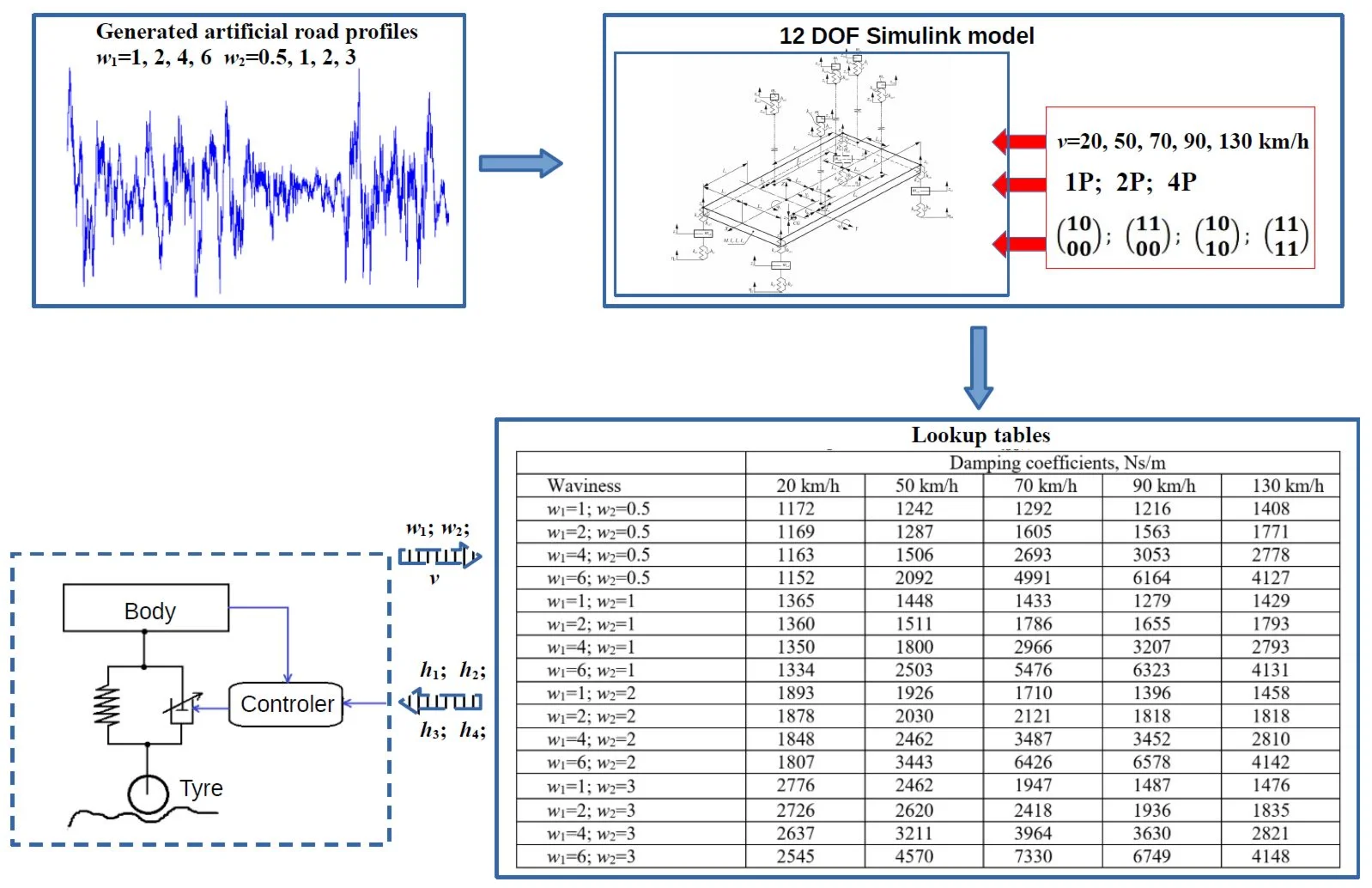
2.1. Road profiles

Real experiments require the measurement of the road profile. Different direct, non-contact measurements or system response-based estimations can be used. For simulation, it was possible to use a measured real road profile or a generated artificial profile with the prescribed parameters. An artificial random road profile can be generated through the implementation of 1) linear filtering, 2) superposition of harmonics (sinusoidal approximation), and 3) inverse fast Fourier transform of discretized power spectral density (PSD) [75]. We also used one of the most commonly implemented methods [76]-[78] for superposition of harmonics. Longitudinal road profiles were generated using the original MATLAB^TM code, implementing the method of superposition of harmonics in the spatial domain according to Eqs. (1-2):

1

z (x) = \sum_{i = 1}^{N = (Ω_{U} - Ω_{L}) / Δ Ω} Z_{i} \cos (Ω_{i} x + φ_{i}),

2

Z_{i} = \sqrt{2 G_{d} (Ω_{i}) Δ Ω},

where $Z_{i}$ , $Ω_{i} = Ω_{L} + (i - 1) Δ Ω$ , $φ_{i}$ are respectively amplitude, angular spatial frequency and uniformly distributed phase angle of $i$ th harmonic; $Ω_{U}$ , $Ω_{L}$ , $Δ Ω$ are respectively upper or lower angular spatial frequencies in the PSD spectrum and the width of each frequency band; $G_{d} (Ω_{i})$ is displacement PSD at the angular spatial frequency $Ω_{i}$ ; $N$ is number of harmonics (we used 1000). The ISO 8608 standard recommends the lower and upper limits of the angular spatial frequencies (= 2 $π n$ ) equal to 2 $π$ ×0.01 rad/m and 2 $π$ ×10 rad/m for general on-road measurements, respectively [79]. In order to generate different road profiles that match the real roads more closely, we replaced the linear fitting of $G_{d} (Ω)$ proposed by ISO [79] to two split fittings offered by P. Andrén [80] in Eq. (2) and modified it by reducing the amplitude of frequencies higher than $Ω_{2}$ and lower than 0.04×2 $π$ rad/m:

3

G_{d} (Ω) = \{\begin{array}{l} G_{d} (Ω_{0}) Ω^{- 1}, & Ω \leq 0.04 \times 2 π r a d / m, \\ G_{d} (Ω_{0}) Ω^{- w_{1}}, & 0.04 \times 2 π r a d / m \leq Ω \leq Ω_{2}, \\ G_{d} (Ω_{0}) Ω^{- w_{2}}, & Ω_{1} \leq Ω \leq Ω_{2}, \\ G_{d} (Ω_{0}) Ω^{- w_{3} = 5}, & Ω_{2} \leq Ω, \end{array}

where $w_{i}$ is waviness; $Ω_{0} =$ 1 rad/m, $Ω_{1} =$ 0.21×2 $π$ rad/m and $Ω_{2} =$ 1.22×2 $π$ rad/m. These values of reference, lower, and higher break frequencies, respectively, produced a minimal error for the Swedish road network [80]. In addition, Welch-type window functions have been used to minimize the appearance of sudden shifts in connections between profile segments, with 10 exponential values [81]. The left-hand wheels passed the profile generated in this way, while for the right-hand wheels it was modified by randomly increasing or decreasing it values up to 20 %. An identical random number sequence was used to generate each profile for comparison.

2.2. Dynamic model

The dynamic response of Range Rover Evoque to road irregularities was analyzed using a full-car model with 12 DOFs [82]: seven DOFs for the vehicle body [21] and five DOFs for vertical displacements along the $Z$ -axis of the crew and baggage box masses. In other words, our model included 10 masses (car body, four wheels, driver, three passengers, and baggage box) and two moments of inertia about the $X$ and $Y$ axes and was constructed using Lagrange’s equation of the second type in generalized coordinates. These equations were solved analytically, and after differentiation the final system was obtained, which consists of 12 equations presented in this way:

4

a_{i i} {\ddot{q}}_{i} + b_{i 1} {\dot{q}}_{1} + b_{i 2} {\dot{q}}_{2} + \dots + b_{i n} {\dot{q}}_{n} + c_{i 1} q_{1} + c_{i 2} q_{2} + \dots + c_{i n} q_{n}

= d_{i 1} η_{1} + d_{i 2} η_{2} + d_{i 3} η_{3} + d_{i 4} η_{4} + d_{i 1}^{*} {\dot{η}}_{1} + d_{i 2}^{*} {\dot{η}}_{2} + d_{i 3}^{*} {\dot{η}}_{3} + d_{i 4}^{*} {\dot{η}}_{4},

where $a$ , $b$ , $c$ , $d$ and $d^{*}$ (with corresponding indexes) are coefficients of equations derived from matrices of stiffness, dissipation, and inertia; $q_{i}$ is a generalized coordinate applied to the formation of the equation system; $n$ is the number of generalized coordinates or DOFs; and $η_{1}$ , $η_{2}$ , $η_{3}$ , $η_{4}$ are coordinates along which the car system is kinetically excited. More information about our model and its derivation can be found in [82]. The road profiles generated as above were used as input. When passing the corresponding profiles, the front and rear wheels were excited by road irregularities located at a distance equal to the distance between the axle centers.

The same ( $h_{s F 1} = h_{s F 2} = h_{s R 1} = h_{s R 2}$ ), two different values for the front and rear ( $h_{s F 1} = h_{s F 2}$ , $h_{s R 1} = h_{s R 2}$ ), or all different damping coefficients ( $h_{s F 1}$ , $h_{s F 2}$ , $h_{s R 1}$ , $h_{s R 2}$ ) for all wheels, which define the behavior of the suspension, were optimized as parameters (marked as 1P, 2P, and 4P, respectively) to reach the minimal RMS value of the vertical acceleration of the crew. In other words, the suspension system was adjusted for the maximum driver, for the driver and front passenger, for the driver and rear left passenger, and for the entire crew comfort. The mathematical solution of Eq. (4) and the optimization process were processed using Simulink/MATLAB^TM software and its response optimization, using the Gradient Descent method. The response optimization tool was configured to optimize the damping coefficients as parameters to find the minimum final value of the RMS of the vertical acceleration passing through the entire road profile. The objective function was constructed using the RMS value of the vertical acceleration for the driver, or their sum for the driver and front passenger, for the driver and rear left passenger, and for the entire crew, respectively, with default weighting value 1. All elements of the suspension system, tire stiffness, and damping were assumed to be linear [53]. During optimization, the damping coefficient can vary from a minimum of 1000 Ns/m to a maximum of 15000 Ns/m. The masses of the crew were chosen as 100 kg, 80 kg, 60 kg, and 40 kg for the driver, front passenger, rear right passenger, and rear left passenger, respectively. The other parameters were the same as those used in Ref. [82].

3. Results and discussion

Initially, we generated road profiles with waviness $w_{1}$ values of 1, 2, 4, and 6; w₂ values of 0.5, 1, 2, and 3; and value of displacement PSD for ISO road class B $G_{d} (Ω_{0}) =$ 4×10^-6 m³ [79]. The length of the longitudinal road profile was 200 m. It is twice as much as needed to accommodate the ISO 8608 standard recommended the lower limits of the spatial frequency equal to 0.01 cycle/m. Using our dynamic full-car model, we had been simulating a vehicle passing these profiles at speeds $v =$ 20, 50, 70, 90, and 130 km/h. When optimized for the driver and the same damping for all wheels, the values of the damping coefficient of the optimized suspension for the generated profiles and various speeds are shown in Table 1 and in Tables A1-A3, respectively, when optimized for the driver and front passenger, for the driver and rear left passenger, or for the whole crew.

Table 1Dependence of the damping on vehicle speed and road waviness (Cases: one coefficient (1P), optimization for driver (0 01 0))

	Damping coefficients, Ns/m
Waviness	20 km/h	50 km/h	70 km/h	90 km/h	130 km/h
$w_{1} =$ 1; $w_{2} =$ 0.5	1172	1242	1292	1216	1408
$w_{1} =$ 2; $w_{2} =$ 0.5	1169	1287	1605	1563	1771
$w_{1} =$ 4; $w_{2} =$ 0.5	1163	1506	2693	3053	2778
$w_{1} =$ 6; $w_{2} =$ 0.5	1152	2092	4991	6164	4127
$w_{1} =$ 1; $w_{2} =$ 1	1365	1448	1433	1279	1429
$w_{1} =$ 2; $w_{2} =$ 1	1360	1511	1786	1655	1793
$w_{1} =$ 4; $w_{2} =$ 1	1350	1800	2966	3207	2793
$w_{1} =$ 6; $w_{2} =$ 1	1334	2503	5476	6323	4131
$w_{1} =$ 1; $w_{2} =$ 2	1893	1926	1710	1396	1458
$w_{1} =$ 2; $w_{2} =$ 2	1878	2030	2121	1818	1818
$w_{1} =$ 4; $w_{2} =$ 2	1848	2462	3487	3452	2810
$w_{1} =$ 6; $w_{2} =$ 2	1807	3443	6426	6578	4142
$w_{1} =$ 1; $w_{2} =$ 3	2776	2462	1947	1487	1476
$w_{1} =$ 2; $w_{2} =$ 3	2726	2620	2418	1936	1835
$w_{1} =$ 4; $w_{2} =$ 3	2637	3211	3964	3630	2821
$w_{1} =$ 6; $w_{2} =$ 3	2545	4570	7330	6749	4148

The use of one damping value for all wheels in the full-car model was similar to the use of the quarter-car model. Nevertheless, the advantage is that we can optimize for different combinations of passenger positions and also consider pitch and roll dynamics and the influence of separate wheels. The dependencies of the optimized damping coefficient on the waviness $w_{1}$ , $w_{2}$ and speed are the same as those observed to optimize suspensions with various locations of masses [74]. The optimal damping values increased when both waviness indices increased, except when the speed was equal to 20 km/hand $w_{1}$ increased. The highest damping values occurred when $w_{1} =$ 6 and the speed was 70 km/h or 90 km/h. Higher damping values are required to increase $w_{2}$ at a fixed $w_{1}$ , and this difference changes from thousands to tens with increasing speed. When fixed $w_{2}$ , the damping differences owing to the change in $w_{1}$ increased with increasing speed and reached a maximum at speeds of 70 km/h or 90 km/h. However, higher damping is also required when the optimization purpose is for the driver with the rear left passenger or whole crew compared to the optimization for the driver or for the driver with the front passenger. This is because rear suspensions require higher damping (see below).

Table 2Dependence of the damping on vehicle speed and road waviness (Cases: two different coefficient for front and rear (2P), respectively, top and bottom values, optimization for driver and rear left passenger (1 01 0))

	Damping coefficients, Ns/m
Waviness	20 km/h	50 km/h	70 km/h	90 km/h	130 km/h
$w_{1} =$ 1; $w_{2} =$ 0.5	1100 2444	1173 2164	1000 3426	1000 2770	1228 2570
$w_{1} =$ 2; $w_{2} =$ 0.5	1103 2404	1157 2746	1000 4976	1134 4610	1579 2786
$w_{1} =$ 4; $w_{2} =$ 0.5	1106 2335	1102 5165	1092 10022	1542 8163	2497 3451
$w_{1} =$ 6; $w_{2} =$ 0.5	1108 2251	1000 12291	1491 15000	3908 11078	3698 3833
$w_{1} =$ 1; $w_{2} =$ 1	1248 3117	1361 2702	1002 4029	1050 3193	1233 2740
$w_{1} =$ 2; $w_{2} =$ 1	1253 3067	1330 3536	1096 5713	1177 5091	1583 2949
$w_{1} =$ 4; $w_{2} =$ 1	1257 2942	1243 6680	1230 10460	1664 8287	2506 3513
$w_{1} =$ 6; $w_{2} =$ 1	1258 2839	1120 14389	1829 15000	4196 11168	3699 3847
$w_{1} =$ 1; $w_{2} =$ 2	1622 4842	1790 3991	1216 4948	1114 3871	1236 2948
$w_{1} =$ 2; $w_{2} =$ 2	1631 4768	1732 5223	1310 6675	1268 5619	1593 3135
$w_{1} =$ 4; $w_{2} =$ 2	1632 4555	1588 9283	1554 10918	1874 8428	2517 3580
$w_{1} =$ 6; $w_{2} =$ 2	1629 4254	1482 15000	2616 15000	4621 11279	3706 3857
$w_{1} =$ 1; $w_{2} =$ 3	2208 6880	2278 5115	1399 5525	1169 4284	1237 3060
$w_{1} =$ 2; $w_{2} =$ 3	2197 6731	2181 6521	1526 7199	1349 5931	1598 3213
$w_{1} =$ 4; $w_{2} =$ 3	2206 6528	1981 10891	1877 11132	2027 8506	2526 3608
$w_{1} =$ 6; $w_{2} =$ 3	2182 6080	1924 15000	3457 15000	4894 11323	3711 3863

A more realistic case in a vehicle is when different damping values are used for the front and rear suspensions. Such optimized results are presented in Table 2, optimizing for driver and rear left passenger or Tables A4-A6 optimizing for driver, driver and front passenger, and for the entire crew, respectively. Other results of more complex cases where all damping are different are shown in Table 3 optimizing for the whole crew or Tables A7-A9 optimizing for the driver, for the driver and front passenger, and for the driver and rear left passenger, respectively. The above-mentioned tendencies of dependencies of optimized damping are observed in cases with two and four different damping values with few peculiarities. Rear suspensions require higher damping values than front suspensions because of their larger share of total mass. The rear damping values do not increase but decrease with increasing waviness, but only if optimized for the driver or driver and front passenger (see Tables A4, A5, A7, A8). The highest damping values when $w_{1} =$ 6 shifted to a lower speed range (50 km/h or 70 km/h). There are situations where the limit damping values are reached, especially a lot of times when the speed is 50 km/h and 70 km/h and optimized for the driver or driver and front passenger. Here, one can observe the tendency that lower damping is required when the optimization purpose is the driver with rear left passenger or whole crew, compared with the optimization for the driver or for the driver with the front passenger (opposite to one damping value).

Table 3Dependence of the damping on vehicle speed and road waviness (Cases: four different coefficients (4P) (top left is front left and bottom right is rear right), optimization for driver and all passengers (1 11 1))

	Damping coefficients, Ns/m
Waviness	20 km/h	50 km/h	70 km/h	90 km/h	130 km/h
$w_{1} =$ 1; $w_{2} =$ 0.5	1000 1068 2400 3186	1085 1123 2213 2750	1000 1000 3539 4444	1000 1000 3004 3823	1000 1319 2282 4357
$w_{1} =$ 2; $w_{2} =$ 0.5	1000 1071 2365 3146	1033 1124 2804 3645	1000 1000 5226 6592	1000 1000 5054 6373	1000 1915 2202 5508
$w_{1} =$ 4; $w_{2} =$ 0.5	1000 1076 2294 3070	1000 1040 5694 6886	1000 1000 10129 11948	1472 1183 8304 8967	1000 3581 1940 6740
$w_{1} =$ 6; $w_{2} =$ 0.5	1000 1081 2199 2966	1000 1000 13678 14830	1314 1150 15000 15000	4725 1509 10442 11128	1789 5115 2337 6190
$w_{1} =$ 1; $w_{2} =$ 1	1056 1243 3087 4002	1238 1316 2852 3416	1000 1000 4336 5170	1000 1000 3598 4416	1000 1325 2420 4545
$w_{1} =$ 2; $w_{2} =$ 1	1058 1246 3027 3941	1196 1290 3804 4532	1000 1000 6188 7450	1000 1082 5523 6794	1000 1943 2278 5639
$w_{1} =$ 4; $w_{2} =$ 1	1067 1247 2938 3814	1092 1188 7719 8625	1106 1008 10690 12226	1594 1285 8451 8933	1000 3607 1942 6764
$w_{1} =$ 6; $w_{2} =$ 1	1071 1254 2806 3675	1000 1065 15000 15000	1596 1366 15000 15000	2512 5861 12267 9470	1815 5097 2362 6198
$w_{1} =$ 1; $w_{2} =$ 2	1460 1575 4894 5536	1616 1784 4567 4636	1088 1109 5577 6167	1000 1013 4514 5277	1000 1322 2621 4765
$w_{1} =$ 2; $w_{2} =$ 2	1456 1576 4763 5417	1550 1720 6015 6112	1158 1161 7352 8209	1106 1154 6139 7139	1000 1974 2374 5777
$w_{1} =$ 4; $w_{2} =$ 2	1458 1580 4583 5191	1391 1554 10687 10722	1379 1325 11269 11988	1799 1501 8637 8852	1000 3634 1945 6795
$w_{1} =$ 6; $w_{2} =$ 2	1463 1592 4374 4980	1356 1427 15000 15000	2323 2024 15000 15000	3128 5959 12296 9603	1843 5097 2390 6197
$w_{1} =$ 1; $w_{2} =$ 3	2023 2243 7139 7116	2002 2410 6168 5347	1267 1298 6307 6544	1000 1124 4959 5720	1000 1321 2740 4869
$w_{1} =$ 2; $w_{2} =$ 3	2033 2247 6886 6925	1914 2299 7820 6932	1366 1387 7998 8376	1200 1229 6476 7276	1000 1991 2427 5842
$w_{1} =$ 4; $w_{2} =$ 3	2036 2215 6604 6612	1714 2054 12652 11419	1671 1690 11734 11679	1948 1704 8750 8791	1000 3647 1947 6809
$w_{1} =$ 6; $w_{2} =$ 3	1997 2234 6333 6281	1809 1842 15000 15000	3156 2836 15000 15000	3529 6145 12338 9680	1860 5089 2406 6197

More actual information is how all these changes influence ride comfort (in our case, the RMS of the vertical acceleration). We compared the RMS values on different sides of view to answer the question of what is the most suitable for ensuring the best ride comfort for all crews. First, we compared the percentage changes in the RMS value of vertical acceleration (for all four positions and the sum) relative to the reference of the corresponding RMS values of vertical acceleration for the corresponding speed and road profile when optimized for the driver. It was calculated as follows (using this equation, positive values indicate a percentage increase, whereas negative values indicate a percentage decrease):

5

% c h a n g e = \frac{v a l u e - r e f e r e n c e}{r e f e r e n c e} \times 100 .

The maximum decrease and increase in the percentage change for the cases with one, two, or four damping coefficients and different optimizations are shown in Table 4 relative to the reference of the corresponding RMS values of vertical acceleration for the corresponding speed and road profile when optimized for the driver with the same number of damping values. The dependences of these reference values of the sum of the RMS value of the vertical accelerations of the entire crew on the $w_{1}$ and $w_{2}$ waviness of the road profile when the vehicle speed is 20 km/h, 50 km/h, 70 km/h, 90 km/h, or 130 km/h are shown in Fig. 1 (or in Figs. A1-A4 for separate passengers). These dependencies of the reference values have the same common tendencies, and it is obvious that they have slightly different values. From the point of view of the optimization purpose relative to the optimization for the driver (Table 4), the sum of the RMS values decreased for all road profiles and speed values only if the optimization purpose was the entire crew using one, two, or four damping values as parameters (maximum down to –15 % or –0.58 m/s²). However, for example, the percentage change of –13.7 % corresponds to –0.89 m/s² or –0.55 m/s² difference, or –7.36 % to –0.77 m/s². In general, there is no correlation between the values of percentage change and the values of difference (compare the results in Table 4 and Table A10 or Table A11 and Table A12), and the minimum and maximum values of difference and percentage change appear in different situations. A comparison of the dependences of the percentage change and difference on the road profile and speed for the two cases with the sum of the RMS is shown in Fig. 2. Only the zero values (blue lines in Fig. 2) were in the same location. Although the sum of the RMS values decreased for all road profiles and speed values when the optimization purpose was the entire crew using four damping values, a detailed analysis of the full data showed that the improvement in comfort is observed only for two or three passengers simultaneously, and it is one point ( $w_{1} =$ 1, $w_{2} =$ 1, $v =$ 70 km/h), where it improves for the driver. It is known from previous work [33], [74] that when changing the optimization purpose from only the driver to other purposes, we increase the comfort level for others but decrease it for the driver.

Table 4The maximum percentage change in the RMS value of vertical acceleration (for the four positions and the sum) relative to the reference of the corresponding RMS values of vertical acceleration for the corresponding speed and road profile when optimized for the driver with the same number of damping values. FL – front left (driver), FR – front right passenger, RL – rear left passenger, RR – rear right passenger

Damping values		Percentage change, %
Damping values	Optimized for		RMS( $a_{F L}$ )	RMS( $a_{F R}$ )	RMS( $a_{R R}$ )	RMS( $a_{R L}$ )	$Σ$ RMS
1P	$(_{0 0}^{1 0}$ )	as reference
	$(_{0 0}^{1 1}$ )	min	0.00	–0.69	–0.90	–0.89	–0.51
	$(_{0 0}^{1 1}$ )	max	0.26	0.00	2.55	2.28	1.08
	$(_{1 0}^{1 0}$ )	min	0.02	–0.24	–19.9	–18.7	–6.88
	$(_{1 0}^{1 0}$ )	max	9.06	8.31	–0.03	–0.04	0.09
	$(_{1 1}^{1 1}$ )	min	0.01	-0.36	–20.7	–19.5	–6.90
	$(_{1 1}^{1 1}$ )	max	10.1	9.20	0.14	0.10	–0.00
2P	$(_{0 0}^{1 0}$ )	as reference
	$(_{0 0}^{1 1}$ )	min	–0.69	–2.55	–8.66	–8.21	–5.39
	$(_{0 0}^{1 1}$ )	max	0.52	0.00	1.73	1.98	0.81
	$(_{1 0}^{1 0}$ )	min	–0.24	–0.06	–33.7	–34.4	–14.9
	$(_{1 0}^{1 0}$ )	max	14.1	12.6	–0.18	–0.28	0.09
	$(_{1 1}^{1 1}$ )	min	–0.30	–0.15	–33.2	–33.9	–15.1
	$(_{1 1}^{1 1}$ )	max	14.1	12.0	0.02	–0.04	–0.01
4P	$(_{0 0}^{1 0}$ )	as reference
	$(_{0 0}^{1 1}$ )	min	–1.05	–24.2	–15.6	–7.58	–7.36
	$(_{0 0}^{1 1}$ )	max	11.9	0.06	23.2	11.0	3.95
	$(_{1 0}^{1 0}$ )	min	–0.01	–17.5	–29.9	–35.8	–13.7
	$(_{1 0}^{1 0}$ )	max	27.9	31.7	16.6	–1.13	4.76
	$(_{1 1}^{1 1}$ )	min	–0.00	–18.5	–31.7	–32.8	–13.7
	$(_{1 1}^{1 1}$ )	max	10.5	10.7	4.92	3.64	–0.00

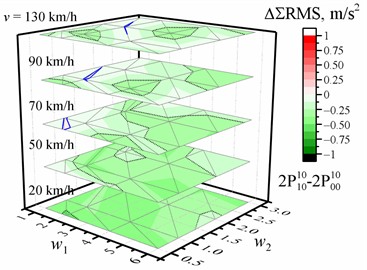
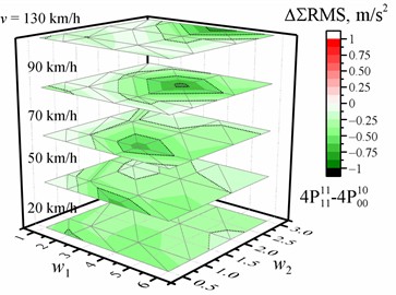
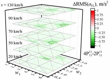
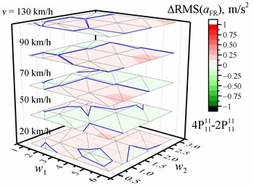
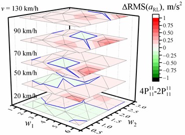
The dependence of the difference in the RMS value of the vertical acceleration of the separate passengers on the $w_{1}$ and $w_{2}$ waviness of the road profile and vehicle speed is shown in Fig. 3 for the case optimized for the entire crew with four damping values relative to the reference when optimized for the driver with four damping values. In all calculated situations, there are only a few situations where comfort is improved for the entire crew (see Table 5) compared to optimization for the driver. Most of them occur when we change the optimization purpose from the driver to the driver with the front-right passenger. The highest increases in comfort for separate passengers are from 30 % to 36 % for rear passengers when optimized for the driver and rear left passenger or for the entire crew with two or four damping values (RMS values decrease in the range from –0.35 m/s² to –1 m/s²).

Fig. 1Dependence of the sum of the RMS values of the vertical accelerations of the entire crew on the w1 and w2 waviness of the road profile and the vehicle speed v. The black dotted line shows the major tick value

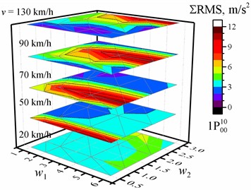
a) Optimized for the driver with one damping value

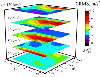
b) Optimized for the driver with two damping values

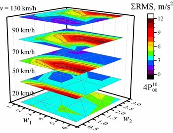
c) Optimized for the driver with four damping values

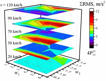
d) Optimized for the entire crew with four damping values

Fig. 2Dependence of the percentage change (a, b) / difference (c, d) in the sum of the RMS values of vertical accelerations of the entire crew on the w1 and w2 waviness of the road profile and the vehicle speed v relative to the reference of the corresponding sum of the RMS values of vertical accelerations for the corresponding speed and road profile when optimized for the driver, respectively, with two or four damping values. The black dotted line shows the major tick value. The solid blue line is zero

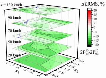
a) Optimized for the driver and rear left passenger with two damping values

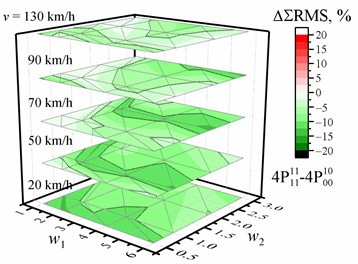
b) Optimized for the entire crew with four damping values

c) Optimized for the driver and rear left passenger with two damping values

d) Optimized for the entire crew with four damping values

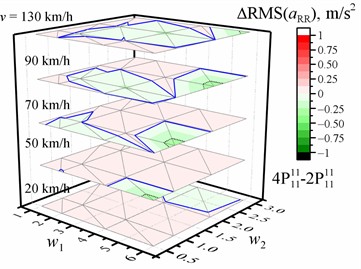
Fig. 3Dependence of the difference in the RMS value of the vertical acceleration (a, b, c, d) on the w1 and w2 waviness of the road profile and the vehicle speed v when optimized for the entire crew with four damping values relative to the reference of the corresponding RMS values of vertical accelerations for the corresponding speed and road profile when optimized for the driver with four damping values. The black dotted line shows the major tick value. The solid blue line is zero

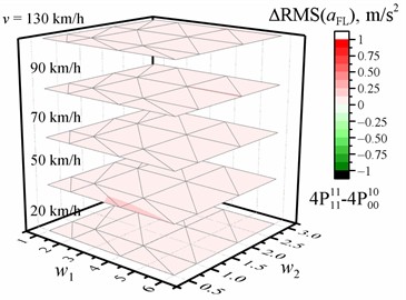
a) Of the driver (front left)

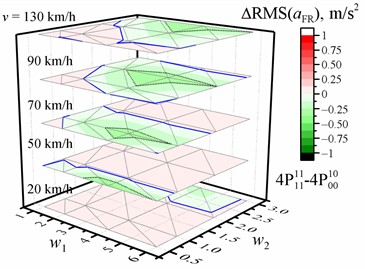
b) Of the front right passenger

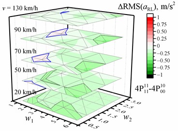
c) Of the rear left passenger

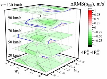
d) Of the rear right passenger

The comparison results relative to the optimization for the entire crew with four damping values are presented in Table 6. Here, we show the average percentage change over all profiles and velocities. From these results, we can state that the optimization for the entire crew with only four damping values is not the best choice for all passengers in all cases. Negligible changes in the increase and decrease in the sum of the RMS were obtained when optimized for the driver and rear left passenger or the entire crew with two damping values compared with the case of the entire crew with four damping values (see Table A11). These three cases had nearly the same average sum of the RMS averaged over all profiles and velocities.

Table 5Points where comfort increases for the entire crew relative to the reference when optimized for the driver with the same number of damping values

Cases	$w_{1}$	$w_{2}$	$v$ , km/h	$∆ Σ$ RMS, m/s²	$∆ Σ$ RMS, %
$4 P_{00}^{11} - 4 P_{00}^{10}$	1	2	50	–0.00011	–0.0033
	1	3	50	–0.140	–3.9
	6	2	70	–0.00014	–0.0049
	1	0.5	90	–0.137	–4.3
$2 P_{11}^{11} - 2 P_{00}^{10}$	6	2	130	–0.014	–1.7
$2 P_{10}^{10} - 2 P_{00}^{10}$	6	2	130	–0.014	–1.7
$2 P_{00}^{11} - 2 P_{00}^{10}$	1	2	20	–0.147	–3.7
	6	3	20	–0.017	–0.48
	1	3	50	–0.14	–4.1
	2	3	50	–0.21	–5.4
	1	3	70	–0.00032	–0.01
	1	0.5	90	-0.14	–4.4
	2	0.5	130	–0.0006	–0.078
	6	2	130	–0.0026	–0.3

Fig. 4 shows the dependence of the difference in the RMS value of the vertical accelerations on the waviness $w_{1}$ and $w_{2}$ of the road profile and the vehicle speed when optimized for the entire crew with four damping values relative to the reference of the corresponding RMS values of the vertical accelerations for the corresponding speed and road profile when optimized for the entire crew with two damping values. It can be seen that only for the driver is better optimization with four damping values. This could be explained by the fact that, when optimized for the entire crew with four damping values, we sometimes reached the limit values. We believe that better comfort results will be obtained if during optimization 1) we would check the minimal value separately for all passengers; 2) we would change not only damping, but also stiffness, or would use asymmetric suspensions or non-linear models; and 3) we would limit the highest values of acceleration. The comfort level is very low when the magnitude of the total values of the overall vibration ranges from 1.25 m/s² to 2.5 m/s² and extremely uncomfortable when they are even greater [66]. When the acceleration value is still high even after optimization, we could also additionally recommend reducing the speed. Therefore, by combining information from vehicle sensors about speed, masses with their location and information stored in a microcomputer or cloud about optimal damping, vertical acceleration, and road information, we can control damping and recommend or reduce driving speed [83], [84]. Using real-time data, the required damping value could be interpolated from 3D lookup tables of optimized damping coefficients calculated at our fixed values of speed v and waviness indices $w_{1}$ , $w_{2}$ by applying different optimization strategies.

Comparing our four optimization tasks, we can conclude that optimization for the driver and for the driver and front-right passenger gives similar results with one damping value. However, the percentage change increases with an increasing number of damping values. When comparing the optimization for the driver and rear-left passenger and for the entire crew, one has nearly similar values, except for the case with four damping values, where the larger changes are. This could be related to the higher comfort level of the crew. Finally, we could recommend to use one damping value when the speed of calculation is required for a short time (e.g., detected bump on the road). Add more regimes, for example, ‘taxi,’ when optimized for the driver because he rides all day and the passengers only ride for a short time, or ‘trip’ when optimized for the entire crew.

Table 6The average over all profiles and velocities of percentage change in the RMS value of vertical acceleration (for all four positions and the sum) relative to the reference of the corresponding RMS values of vertical acceleration for the corresponding speed and road profile when optimized for the entire crew (1 11 1) with four damping values (4P). FL – front left (driver), FR – front right passenger, RL – rear left passenger, RR – rear right passenger

Damping values		Average of percentage change, %
Damping values	Optimized for	RMS( $a_{F L}$ )	RMS( $a_{F R}$ )	RMS( $a_{R R}$ )	RMS( $a_{R L}$ )	$Σ$ RMS
1P	$(_{0 0}^{1 0}$ )	16.1	12.3	12.1	7.08	11.7
	$(_{0 0}^{1 1}$ )	16.2	12.1	12.6	7.56	11.9
	$(_{1 0}^{1 0}$ )	19.6	15.8	3.55	–0.82	9.10
	$(_{1 1}^{1 1}$ )	19.9	15.9	3.41	–0.95	9.09
2P	$(_{0 0}^{1 0}$ )	–1.44	–4.89	20.0	19.0	6.95
	$(_{0 0}^{1 1}$ )	–1.38	–5.18	19.5	18.6	6.64
	$(_{1 0}^{1 0}$ )	3.83	–0.05	–0.56	–2.65	0.01
	$(_{1 1}^{1 1}$ )	3.40	–0.84	–0.15	–2.08	–0.06
4P	$(_{0 0}^{1 0}$ )	–4.09	0.51	17.6	18.0	7.01
	$(_{0 0}^{1 1}$ )	–2.34	–4.76	18.8	18.8	6.50
	$(_{1 0}^{1 0}$ )	2.13	5.42	3.35	–4.10	1.49
	$(_{1 1}^{1 1}$ )	As reference

Fig. 4Dependence of the difference in the RMS value of the vertical acceleration (a, b, c, d) on the w1 and w2 waviness of the road profile and the vehicle speed v when optimized for the entire crew with four damping values relative to the reference of the corresponding RMS values of vertical accelerations for the corresponding speed and road profile when optimized for the entire crew with two damping values. The black dotted line shows the major tick value. The solid blue line is zero

a) Of the driver (front left)

b) Of the front right passenger

c) Of the rear left passenger

d) Of the rear right passenger

4. Conclusions

The relationship between the detected road waviness values and optimized damping coefficient can be used to control the damping of the suspension system and recommend or reduce the driving speed. The required optimized damping value could be interpolated from a 3D gridded matrix of damping coefficients calculated at certain fixed values of speed and waviness indices when optimized with the same, two different for the front and rear, or all different damping coefficients for all wheels and using different optimization strategies. Our simulation results showed that higher damping is required when the optimization purpose is for the driver with the rear left passenger or the entire crew compared to the optimization for the driver or for the driver with the front passenger. In addition, optimization by changing only two or four different damping coefficients in the suspension system is not sufficient because there are too many cases where it reaches limit values.

From the point of view of the optimization purpose relative to the optimization for the driver, the sum of the RMS values decreases for all road profiles and speed values only if the optimization purpose is the entire crew using one, two, or four damping values as parameters (maximum down to –15 %). Comparing the optimization for the driver and rear-left passenger and for the entire crew, we obtained similar values, except for the case with four damping values, where larger changes were observed. However, the optimization for the entire crew with four damping values is not the best choice for all situations. Furthermore, we could recommend two regimes like ‘taxi’ and ‘trip’ where the comfort level is optimized for the driver or the entire crew, respectively.

For future improvement, we believe that better results will be obtained if 1) we would change not only damping but also stiffness or would use asymmetric suspensions or nonlinear models; 2) we would check the minimal value separately for all passengers during optimization; and 3) we would control the highest values of acceleration reducing speed.

References

P. S. Els, N. J. Theron, P. E. Uys, and M. J. Thoresson, “The ride comfort vs. handling compromise for off-road vehicles,” Journal of Terramechanics, Vol. 44, No. 4, pp. 303–317, Oct. 2007, https://doi.org/10.1016/j.jterra.2007.05.001

Publisher
J. Zhu, W. Zhang, and M. X. Wu, “Evaluation of ride comfort and driving safety for moving vehicles on slender coastal bridges,” Journal of Vibration and Acoustics, Vol. 140, No. 5, p. 05101, Oct. 2018, https://doi.org/10.1115/1.4039569

Publisher
T. Li, Vehicle/Tire/Road Dynamics: Handling, Ride, and NVH. Elsevier, 2022.

Search CrossRef
D. Karnopp, “Active damping in road vehicle suspension systems,” Vehicle System Dynamics, Vol. 12, No. 6, pp. 291–311, Jul. 2007, https://doi.org/10.1080/00423118308968758

Publisher
R. S. Sharp and D. A. Crolla, “Road vehicle suspension system design – a review,” Vehicle System Dynamics, Vol. 16, No. 3, pp. 167–192, Jan. 1987, https://doi.org/10.1080/00423118708968877

Publisher
D. Fischer and R. Isermann, “Mechatronic semi-active and active vehicle suspensions,” Control Engineering Practice, Vol. 12, No. 11, pp. 1353–1367, Nov. 2004, https://doi.org/10.1016/j.conengprac.2003.08.003

Publisher
Z. Lozia, “The use of a linear quarter-car model to optimize the damping in a passive automotive suspension system – a follow-on from many authors’ works of the recent 40 years,” The Archives of Automotive Engineering – Archiwum Motoryzacji, Vol. 71, No. 1, pp. 39–71, Mar. 2016, https://doi.org/10.14669/am.vol71.art3

Publisher
J. Goszczak, G. Mitukiewicz, B. Radzymiński, A. Werner, T. Szydłowski, and D. Batory, “The study of damping control in semi-active car suspension,” Journal of Vibroengineering, Vol. 22, No. 4, pp. 933–944, Jun. 2020, https://doi.org/10.21595/jve.2020.20578

Publisher
S. Tengler and K. Warwas, “Driver comfort improvement by a selection of optimal springing of a seat,” Czasopismo Techniczne, Vol. 5, pp. 217–235, Jan. 2017, https://doi.org/10.4467/2353737xct.17.083.6440

Publisher
J. K. Nkrumah, K. S. Amedorme, B. Ziblim, and D. I. Offei, “Review of suspension control and simulation of passive, semi-active and active suspension systems using quarter vehicle model,” American Scientific Research Journal for Engineering, Technology, and Sciences, Vol. 90, No. 1, pp. 144–160, Oct. 2022.

Search CrossRef
P. Barak, “Passive versus active and semi-active suspension from theory to application in north American industry,” SAE Technical Paper 922140, Sep. 1992.

Publisher
I. Ballo, “Comparison of the properties of active and semiactive suspension,” Vehicle System Dynamics, Vol. 45, No. 11, pp. 1065–1073, Nov. 2007, https://doi.org/10.1080/00423110701191575

Publisher
G. Z. Yao, F. F. Yap, G. Chen, W. H. Li, and S. H. Yeo, “MR damper and its application for semi-active control of vehicle suspension system,” Mechatronics, Vol. 12, No. 7, pp. 963–973, Sep. 2002, https://doi.org/10.1016/s0957-4158(01)00032-0

Publisher
D. Karnopp, M. J. Crosby, and R. A. Harwood, “Vibration control using semi-active force generators,” Journal of Engineering for Industry, Vol. 96, No. 2, pp. 619–626, May 1974, https://doi.org/10.1115/1.3438373

Publisher
J. Swevers, C. Lauwerys, B. Vandersmissen, M. Maes, K. Reybrouck, and P. Sas, “A model-free control structure for the on-line tuning of the semi-active suspension of a passenger car,” Mechanical Systems and Signal Processing, Vol. 21, No. 3, pp. 1422–1436, Apr. 2007, https://doi.org/10.1016/j.ymssp.2006.05.005

Publisher
D. Savaresi, F. Favalli, S. Formentin, and S. M. Savaresi, “On-line damping estimation in road vehicle semi-active suspension systems,” IFAC-PapersOnLine, Vol. 52, No. 5, pp. 679–684, Jan. 2019, https://doi.org/10.1016/j.ifacol.2019.09.108

Publisher
S. Lajqi and S. Pehan, “Designs and optimizations of active and semi-active non-linear suspension systems for a terrain vehicle,” Strojniški vestnik – Journal of Mechanical Engineering, Vol. 58, No. 12, pp. 732–743, Dec. 2012, https://doi.org/10.5545/sv-jme.2012.776

Publisher
N. Zhang and Q. Zhao, “Fuzzy sliding mode controller design for semi-active seat suspension with neuro-inverse dynamics approximation for MR damper,” Journal of Vibroengineering, Vol. 19, No. 5, pp. 3488–3511, Aug. 2017, https://doi.org/10.21595/jve.2017.17654

Publisher
L. Z. Ben, F. Hasbullah, and F. W. Faris, “A comparative ride performance of passive, semi-active and active suspension systems for off-road vehicles using half car model,” International Journal of Heavy Vehicle Systems, Vol. 21, No. 1, p. 26, Jan. 2014, https://doi.org/10.1504/ijhvs.2014.057827

Publisher
P. Krauze, “Comparison of control strategies in a semi-active suspension system of the experimental ATV,” Journal of Low Frequency Noise, Vibration and Active Control, Vol. 32, No. 1-2, pp. 67–80, Mar. 2013, https://doi.org/10.1260/0263-0923.32.1-2.67

Publisher
E. M. Elbeheiry and D. C. Karnopp, “Optimization of active and passive suspensions based on a full car model,” International Congress and Exposition, Vol. 104, pp. 1900–1911, Feb. 1995, https://doi.org/10.4271/951063

Publisher
J. Qiao, Y. Choi, and F. Yang, “PSO optimum control strategy of 7 degrees of freedom semi-active suspensions,” Journal of Mechanical Engineering, Automation and Control Systems, Vol. 2, No. 2, pp. 98–108, Dec. 2021, https://doi.org/10.21595/jmeacs.2021.22164

Publisher
S. Chen, H. Chen, and D. Negrut, “Implementation of MPC-based path tracking for autonomous vehicles considering three vehicle dynamics models with different fidelities,” Automotive Innovation, Vol. 3, No. 4, pp. 386–399, Dec. 2020, https://doi.org/10.1007/s42154-020-00118-w

Publisher
S. H. Zareh, A. Sarrafan, A. A. A. Khayyat, and A. Zabihollah, “Intelligent semi-active vibration control of eleven degrees of freedom suspension system using magnetorheological dampers,” Journal of Mechanical Science and Technology, Vol. 26, No. 2, pp. 323–334, Apr. 2012, https://doi.org/10.1007/s12206-011-1007-6

Publisher
S. H. Zareh, M. Abbasi, H. Mahdavi, and K. G. Osgouie, “Semi-active vibration control of an eleven degrees of freedom suspension system using neuro inverse model of magnetorheological dampers,” Journal of Mechanical Science and Technology, Vol. 26, No. 8, pp. 2459–2467, Aug. 2012, https://doi.org/10.1007/s12206-012-0628-8

Publisher
S. Kopylov, Z. Chen, and M. A. A. Abdelkareem, “Implementation of an electromagnetic regenerative tuned mass damper in a vehicle suspension system,” IEEE Access, Vol. 8, pp. 110153–110163, Jan. 2020, https://doi.org/10.1109/access.2020.3002275

Publisher
G. G. Fossati, L. F. F. Miguel, and W. J. P. Casas, “Multi-objective optimization of the suspension system parameters of a full vehicle model,” Optimization and Engineering, Vol. 20, No. 1, pp. 151–177, Sep. 2018, https://doi.org/10.1007/s11081-018-9403-8

Publisher
D. Joshi and A. Deb, “Effect of sitting occupancy on lateral dynamics and trajectory of a passenger car,” in ASME 2015 International Design Engineering Technical Conferences and Computers and Information in Engineering Conference, Vol. 6, Aug. 2015, https://doi.org/10.1115/detc2015-47528

Publisher
A. Deb and D. Joshi, “A study on ride comfort assessment of multiple occupants using lumped parameter analysis,” in SAE 2012 World Congress and Exhibition, Apr. 2012, https://doi.org/10.4271/2012-01-0053

Publisher
H. Du, W. Li, and N. Zhang, “Semi-active control of an integrated full-car suspension with seat suspension and driver body model using ER dampers,” International Journal of Vehicle Design, Vol. 63, No. 2/3, p. 159, Jan. 2013, https://doi.org/10.1504/ijvd.2013.056133

Publisher
V. Guruguntla and M. Lal, “Multi-body modelling and ride comfort analysis of a seated occupant under whole-body vibration,” Journal of Vibration and Control, Vol. 29, No. 13-14, pp. 3078–3095, May 2022, https://doi.org/10.1177/10775463221091089

Publisher
D. Joshi, A. Deb, and C. Chou, “A study on combined effects of road roughness, vehicle velocity and sitting occupancies on multi-occupant vehicle ride comfort assessment,” WCX™ 17: SAE World Congress Experience, Mar. 2017, https://doi.org/10.4271/2017-01-0409

Publisher
P. E. Uys, P. S. Els, and M. Thoresson, “Suspension settings for optimal ride comfort of off-road vehicles travelling on roads with different roughness and speeds,” Journal of Terramechanics, Vol. 44, No. 2, pp. 163–175, Apr. 2007, https://doi.org/10.1016/j.jterra.2006.05.002

Publisher
A. J. Nieto, A. L. Morales, J. M. Chicharro, and P. Pintado, “An adaptive pneumatic suspension system for improving ride comfort and handling,” Journal of Vibration and Control, Vol. 22, No. 6, pp. 1492–1503, Jun. 2014, https://doi.org/10.1177/1077546314539717

Publisher
A. L. Morales, A. J. Nieto, J. M. Chicharro, and P. Pintado, “A semi-active vehicle suspension based on pneumatic springs and magnetorheological dampers,” Journal of Vibration and Control, Vol. 24, No. 4, pp. 808–821, Jun. 2016, https://doi.org/10.1177/1077546316653004

Publisher
A. Hać, “Optimal linear preview control of active vehicle suspension,” Vehicle System Dynamics, Vol. 21, No. 1, pp. 167–195, Jan. 1992, https://doi.org/10.1080/00423119208969008

Publisher
I. Youn and A. Hać, “Semi-active suspensions with adaptive capability,” Journal of Sound and Vibration, Vol. 180, No. 3, pp. 475–492, Feb. 1995, https://doi.org/10.1006/jsvi.1995.0091

Publisher
T.-H. Wu and C.-C. Lan, “A wide-range variable stiffness mechanism for semi-active vibration systems,” Journal of Sound and Vibration, Vol. 363, pp. 18–32, Feb. 2016, https://doi.org/10.1016/j.jsv.2015.10.024

Publisher
R. Tchamna, M. Lee, and I. Youn, “Attitude control of full vehicle using variable stiffness suspension control,” Optimal Control Applications and Methods, Vol. 36, No. 6, pp. 936–952, Nov. 2014, https://doi.org/10.1002/oca.2149

Publisher
C. Spelta et al., “Performance analysis of semi-active suspensions with control of variable damping and stiffness,” Vehicle System Dynamics, Vol. 49, No. 1-2, pp. 237–256, Feb. 2011, https://doi.org/10.1080/00423110903410526

Publisher
V. Goga and M. Kľúčik, “Optimization of vehicle suspension parameters with use of evolutionary computation,” Procedia Engineering, Vol. 48, pp. 174–179, Jan. 2012, https://doi.org/10.1016/j.proeng.2012.09.502

Publisher
R. Jayachandran and S. Krishnapillai, “Modeling and optimization of passive and semi-active suspension systems for passenger cars to improve ride comfort and isolate engine vibration,” Journal of Vibration and Control, Vol. 19, No. 10, pp. 1471–1479, May 2012, https://doi.org/10.1177/1077546312445199

Publisher
H. Huang, S. Sun, S. Chen, and W. Li, “Numerical and experimental studies on a new variable stiffness and damping magnetorheological fluid damper,” Journal of Intelligent Material Systems and Structures, Vol. 30, No. 11, pp. 1639–1652, Apr. 2019, https://doi.org/10.1177/1045389x19844003

Publisher
J. Kumar and G. Bhushan, “Dynamic analysis of quarter car model with semi-active suspension based on combination of magneto-rheological materials,” International Journal of Dynamics and Control, Vol. 11, No. 2, pp. 482–490, Aug. 2022, https://doi.org/10.1007/s40435-022-01024-1

Publisher
A. Soliman and M. Kaldas, “Semi-active suspension systems from research to mass-market – A review,” Journal of Low Frequency Noise, Vibration and Active Control, Vol. 40, No. 2, pp. 1005–1023, Oct. 2019, https://doi.org/10.1177/1461348419876392

Publisher
S. M. Savaresi, C. Poussot-Vassal, C. Spelta, O. Sename, and L. Dugard, Semi-Active Suspension Control Design for Vehicles. Elsevier, 2010, https://doi.org/10.1016/c2009-0-63839-3

Publisher
P. Brezas, M. C. Smith, and W. Hoult, “A clipped-optimal control algorithm for semi-active vehicle suspensions: Theory and experimental evaluation,” Automatica, Vol. 53, pp. 188–194, Mar. 2015, https://doi.org/10.1016/j.automatica.2014.12.026

Publisher
E. Guglielmino, T. Sireteanu, C. W. Stammers, G. Gheorghe, and M. Giuclea, “Semi-active control algorithms,” in Semi-active Suspension Control, London: Springer London, 2024, pp. 65–97, https://doi.org/10.1007/978-1-84800-231-9_4

Publisher
C. Lin, W. Liu, and H. Ren, “State estimation based on unscented Kalman filter for semi-active suspension systems,” Journal of Vibroengineering, Vol. 18, No. 1, pp. 446–457, Feb. 2016.

Search CrossRef
S. Ni and V. Nguyen, “Performance of semi-active cab suspension system with different control methods,” Journal of Mechatronics and Artificial Intelligence in Engineering, Vol. 4, No. 1, pp. 8–17, Jun. 2023, https://doi.org/10.21595/jmai.2022.23019

Publisher
C. Lauwerys, J. Swevers, and P. Sas, “Robust linear control of an active suspension on a quarter car test-rig,” Control Engineering Practice, Vol. 13, No. 5, pp. 577–586, May 2005, https://doi.org/10.1016/j.conengprac.2004.04.018

Publisher
R. Hirao, K. Kasuya, and N. Ichimaru, “A semi-active suspension system using ride control based on bi-linear optimal control theory and handling control considering roll feeling,” SAE 2015 World Congress and Exhibition, Apr. 2015, https://doi.org/10.4271/2015-01-1501

Publisher
I. Ahmad and A. Khan, “A comparative analysis of linear and nonlinear semi-active suspension system,” Mehran University Research Journal of Engineering and Technology, Vol. 37, No. 2, pp. 233–240, Apr. 2018, https://doi.org/10.22581/muet1982.1802.01

Publisher
A. G. Mohite and A. C. Mitra, “Development of linear and non-linear vehicle suspension model,” Materials Today: Proceedings, Vol. 5, No. 2, pp. 4317–4326, Jan. 2018, https://doi.org/10.1016/j.matpr.2017.11.697

Publisher
D. N. L. Horton and D. A. Crolla, “Theoretical analysis of a semi active suspension fitted to an off-road vehicle,” Vehicle System Dynamics, Vol. 15, No. 6, pp. 351–372, Jul. 2007, https://doi.org/10.1080/00423118608968860

Publisher
E. Palomares, J. C. Bellido, A. L. Morales, A. J. Nieto, J. M. Chicharro, and P. Pintado, “Pointwise‐constrained optimal control of a semiactive vehicle suspension,” Optimal Control Applications and Methods, Vol. 42, No. 1, pp. 216–235, Sep. 2020, https://doi.org/10.1002/oca.2671

Publisher
A. Giua, M. Melas, C. Seatzu, and G. Usai, “Design of a predictive semiactive suspension system,” Vehicle System Dynamics, Vol. 41, No. 4, pp. 277–300, Apr. 2004, https://doi.org/10.1080/00423110412331315169

Publisher
G. Li, Z. Ruan, R. Gu, and G. Hu, “Fuzzy sliding mode control of vehicle magnetorheological semi-active air suspension,” Applied Sciences, Vol. 11, No. 22, p. 10925, Nov. 2021, https://doi.org/10.3390/app112210925

Publisher
L. L. Zhao, C. C. Zhou, and Y. W. Yu, “A research on optimal damping ratio control strategy for semi-active suspension system,” Automot. Eng., Vol. 40, No. 2018, pp. 41–47, 2018.

Search CrossRef
A. Hac´ and I. Youn, “Optimal semi-active suspension with preview based on a quarter car model,” Journal of Vibration and Acoustics, Vol. 114, No. 1, pp. 84–92, Jan. 1992, https://doi.org/10.1115/1.2930239

Publisher
J. Theunissen, A. Tota, P. Gruber, M. Dhaens, and A. Sorniotti, “Preview-based techniques for vehicle suspension control: a state-of-the-art review,” Annual Reviews in Control, Vol. 51, pp. 206–235, Jan. 2021, https://doi.org/10.1016/j.arcontrol.2021.03.010

Publisher
M. W. Sayers, T. D. Gillespie, and C. A. V. Queiroz, International Road Roughness Experiment: a Basis for Establishing a Standard Scale for Road Roughness Measurements. Washington, D.C.: World Bank, 1986.

Search CrossRef
M. W. Sayers and S. M. Karamihas, The Little Book of Profiling-Basic Information about Measuring and Interpreting Road Profile. New York, NY, USA: Regent of the University of Michigan, 1998.

Search CrossRef
G. Loprencipe and G. Cantisani, “Unified analysis of road pavement profiles for evaluation of surface characteristics,” Modern Applied Science, Vol. 7, No. 8, pp. 1–14, Jul. 2013, https://doi.org/10.5539/mas.v7n8p1

Publisher
T. Nguyen, B. Lechner, and Y. D. Wong, “Response-based methods to measure road surface irregularity: a state-of-the-art review,” European Transport Research Review, Vol. 11, No. 1, p. 43, Oct. 2019, https://doi.org/10.1186/s12544-019-0380-6

Publisher
“Mechanical vibration and shock – Evaluation of human exposure to whole-body vibration – Part 1: General requirements,” International Organization for Standardization, ISO 2631-1:1997, Jan. 1997.

Search CrossRef
G. Guastadisegni et al., “Ride analysis tools for passenger cars: objective and subjective evaluation techniques and correlation processes – a review,” Vehicle System Dynamics, Vol. 62, No. 7, pp. 1876–1902, Jul. 2024, https://doi.org/10.1080/00423114.2023.2259024

Publisher
G. Papaioannou and D. Koulocheris, “An approach for minimizing the number of objective functions in the optimization of vehicle suspension systems,” Journal of Sound and Vibration, Vol. 435, pp. 149–169, Nov. 2018, https://doi.org/10.1016/j.jsv.2018.08.009

Publisher
Z. Lozia and P. Zdanowicz, “Optimization of damping in the passive automotive suspension system with using two quarter-car models,” in IOP Conference Series: Materials Science and Engineering, Vol. 148, No. 1, p. 012014, Sep. 2016, https://doi.org/10.1088/1757-899x/148/1/012014

Publisher
S. A. Abu Bakar, P. M. Samin, H. Jamaluddin, R. A. Rahman, and S. Sulaiman, “Semi active suspension system performance under random road profile excitations,” in International Conference on Computer, Communications, and Control Technology (I4CT), pp. 93–97, Apr. 2015, https://doi.org/10.1109/i4ct.2015.7219544

Publisher
T. Lenkutis, D. Viržonis, A. Čerškus, A. Dzedzickis, N. Šešok, and V. Bučinskas, “An automotive ferrofluidic electromagnetic system for energy harvesting and adaptive damping,” Sensors, Vol. 22, No. 3, p. 1195, Feb. 2022, https://doi.org/10.3390/s22031195

Publisher
T. Lenkutis et al., “Extraction of information from a PSD for the control of vehicle suspension,” in Automation 2021: Recent Achievements in Automation, Robotics and Measurement Techniques, pp. 146–153, Apr. 2021, https://doi.org/10.1007/978-3-030-74893-7_15

Publisher
A. Čerškus, T. Lenkutis, N. Šešok, A. Dzedzickis, D. Viržonis, and V. Bučinskas, “Identification of road profile parameters from vehicle suspension dynamics for control of damping,” Symmetry, Vol. 13, No. 7, p. 1149, Jun. 2021, https://doi.org/10.3390/sym13071149

Publisher
A. Čerškus, V. Ušinskis, N. Šešok, I. Iljin, and V. Bučinskas, “Optimization of damping in a semi-active car suspension system with various locations of masses,” Applied Sciences, Vol. 13, No. 9, p. 5371, Apr. 2023, https://doi.org/10.3390/app13095371

Publisher
Z. Yonglin and Z. Jiafan, “Numerical simulation of stochastic road process using white noise filtration,” Mechanical Systems and Signal Processing, Vol. 20, No. 2, pp. 363–372, Feb. 2006, https://doi.org/10.1016/j.ymssp.2005.01.009

Publisher
M. Shinozuka and C.-M. Jan, “Digital simulation of random processes and its applications,” Journal of Sound and Vibration, Vol. 25, No. 1, pp. 111–128, Nov. 1972, https://doi.org/10.1016/0022-460x(72)90600-1

Publisher
M. Agostinacchio, D. Ciampa, and S. Olita, “The vibrations induced by surface irregularities in road pavements – a Matlab® approach,” European Transport Research Review, Vol. 6, No. 3, pp. 267–275, Dec. 2013, https://doi.org/10.1007/s12544-013-0127-8

Publisher
C. S. Dharankar, M. K. Hada, and S. Chandel, “Numerical generation of road profile through spectral description for simulation of vehicle suspension,” Journal of the Brazilian Society of Mechanical Sciences and Engineering, Vol. 39, No. 6, pp. 1957–1967, Aug. 2016, https://doi.org/10.1007/s40430-016-0615-6

Publisher
“Mechanical vibration. Road surface profiles. Reporting of measured data,” BSI British Standards, London, ISO 8608:2016(en), Mar. 2022.

Search CrossRef
P. Andren, “Power spectral density approximations of longitudinal road profiles,” International Journal of Vehicle Design, Vol. 40, No. 1/2/3, pp. 2–14, Jan. 2006, https://doi.org/10.1504/ijvd.2006.008450

Publisher
T. Lenkutis, A. Čerškus, N. Šešok, A. Dzedzickis, and V. Bučinskas, “Road surface profile synthesis: assessment of suitability for simulation,” Symmetry, Vol. 13, No. 1, p. 68, Dec. 2020, https://doi.org/10.3390/sym13010068

Publisher
V. Bucinskas, P. Mitrouchev, E. Sutinys, N. Sesok, I. Iljin, and I. Morkvenaite-Vilkonciene, “Evaluation of comfort level and harvested energy in the vehicle using controlled damping,” Energies, Vol. 10, No. 11, p. 1742, Oct. 2017, https://doi.org/10.3390/en10111742

Publisher
J. Wu, H. Zhou, Z. Liu, and M. Gu, “Ride comfort optimization via speed planning and preview semi-active suspension control for autonomous vehicles on uneven roads,” IEEE Transactions on Vehicular Technology, Vol. 69, No. 8, pp. 8343–8355, Aug. 2020, https://doi.org/10.1109/tvt.2020.2996681

Publisher
H. Basargan, A. Mihály, P. Gáspár, and O. Sename, “Cloud-based adaptive semi-active suspension control for improving driving comfort and road holding,” IFAC-PapersOnLine, Vol. 55, No. 14, pp. 89–94, Jan. 2022, https://doi.org/10.1016/j.ifacol.2022.07.588

Publisher

About this article

Received

26 November 2024

Accepted

04 February 2025

Published

05 April 2025

SUBJECTS

Vibration in transportation engineering

DOI

https://doi.org/10.21595/jve.2025.24689

Keywords

semi-active suspension

vehicle damping

optimization

ride comfort

optimization strategy

Acknowledgements

The authors have not disclosed any funding.

Data Availability

The datasets generated during and/or analyzed during the current study are available from the corresponding author on reasonable request.

Author Contributions

Aurimas Čerškus: conceptualization, methodology, validation, formal analysis, investigation, data curation, writing-original draft preparation, writing-review and editing. Nikolaj Šešok: methodology, software, validation, investigation, resources, visualization. Vytautas Bučinskas: conceptualization, writing-review and editing, supervision

Conflict of interest

The authors declare that they have no conflict of interest.

This is an open access article distributed under the Creative Commons Attribution License, which permits unrestricted use, distribution, and reproduction in any medium, provided the original work is properly cited.

Previous article in issue Previous Next article in issue Next

Research article

2023 03 13

Improving ride comfort and road friendliness of heavy truck using semi-active suspension system

Hao Li, Vanliem Nguyen

Research article

2023 01 20

Performance of semi-active cab suspension system with different control methods

Shicheng Ni, Vanliem Nguyen

Research article

2021 12 15

PSO optimum control strategy of 7 degrees of freedom semi-active suspensions

Jubin Qiao, Yeonsung Choi, Fuqiang Yang

Research article

2020 06 30

The study of damping control in semi-active car suspension

Jarosław Goszczak, Grzegorz Mitukiewicz, Bartosz Radzymiński, Andrzej Werner, Tomasz Szydłowski, Damian Batory

A. Čerškus, N. Šešok, and V. Bučinskas, “Implementation of lookup tables for different optimization strategies of semi-active car suspension system,” Journal of Vibroengineering, Vol. 27, No. 3, pp. 497–524, Apr. 2025, https://doi.org/10.21595/jve.2025.24689

Copy Extrica

Copied to clipboard!

TY  - JOUR
DO  - 10.21595/jve.2025.24689
UR  - https://doi.org/10.21595/jve.2025.24689
TI  - Implementation of lookup tables for different optimization strategies of semi-active car suspension system
T2  - Journal of Vibroengineering
AU  - Čerškus, Aurimas
AU  - Šešok, Nikolaj
AU  - Bučinskas, Vytautas
PY  - 2025
DA  - 2025/04/05
PB  - Extrica
SP  - 497-524
VL  - 27
IS  - 3
SN  - 1392-8716
SN  - 2538-8460
ER  - 

Copy Ris

Copied to clipboard!

 @article{_er_kus_2025, title={Implementation of lookup tables for different optimization strategies of semi-active car suspension system}, volume={27}, ISSN={2538-8460}, url={https://doi.org/10.21595/jve.2025.24689}, DOI={10.21595/jve.2025.24689}, number={3}, journal={Journal of Vibroengineering}, publisher={JVE International Ltd.}, author={Čerškus, Aurimas and Šešok, Nikolaj and Bučinskas, Vytautas}, year={2025}, month=apr, pages={497–524} }

Copy Bibtex

Copied to clipboard!

[1]A. Čerškus, N. Šešok, and V. Bučinskas, “Implementation of lookup tables for different optimization strategies of semi-active car suspension system,” Journal of Vibroengineering, vol. 27, no. 3, pp. 497–524, Apr. 2025, doi: 10.21595/jve.2025.24689.

Copy IEEE

Copied to clipboard!

Čerškus, Aurimas, Nikolaj Šešok, and Vytautas Bučinskas. “Implementation of Lookup Tables for Different Optimization Strategies of Semi-Active Car Suspension System.” Journal of Vibroengineering 27, no. 3 (April 5, 2025): 497–524. https://doi.org/10.21595/jve.2025.24689.

Copy Chicago

Copied to clipboard!

Implementation of lookup tables for different optimization strategies of semi-active car suspension system

Abstract

Highlights

1. Introduction

2. Methods

2.1. Road profiles

2.2. Dynamic model

3. Results and discussion

4. Conclusions

References

About this article

Related Articles