Performance evaluation of Compass dual-mode receiver

Zhan, Jianwei; Pang, Jing; Zhang, Guozhu; Ou, Gang

Journal of Vibroengineering

Browse Journal

Submit article

Published: 30 June 2013

Check for updates

Performance evaluation of Compass dual-mode receiver

Jianwei Zhan¹

Jing Pang²

Guozhu Zhang³

Gang Ou⁴

^{1, 2, 3, 4}School of Electronic Science and Engineering, National University of Defense Technology, Changsha 410073, China

Cite the article Download PDF

Downloads 1287

Abstract

Recently, navigation technology based on satellite navigation system has got more and more attention in international society because of its great values for both military and civil application. While navigation signal simulator which can generate satellite navigation signals and simulate different scenarios, not only satisfy cooperating test requirements of ground operation control system, test of the signal receivers, but also been playing a very important role in the development, test and evaluation of different navigation receiver, such as radio determination satellite system (RDSS) receiver, radio navigation satellite system (RNSS) receiver and dual-mode receivers. It is an indispensable tool for the design of the receivers．Compared to other satellite navigation systems, such as Global Positioning System (GPS) and GLobal Navigation Satellite System (GLONASS), BeiDou Navigation Satellite System (Compass/BDS) have some different unique characteristics, especially in RDSS determination. Firstly, the principle of comprehensive RDSS position and report is presented. Then function architecture of Compass signal simulator and requirements of the dynamic navigation signal simulation are analyzed. Finally, two key mathematical models are established to simulate the signals arriving at the receiver antenna for dual-mode receiver test, which are: the transmitting time iterative model and efficient satellite orbit approximation model. The results show that the Compass dual-mode simulator can satisfy dual-mode receiver’s test requirements.

1. Introduction

Beidou satellite navigation system (Compass/BDS) has been providing accurate and continuous three-dimensional (3-D) position, communication and time services since 27th, December, 2012. During the past few years there has been growing interest in Compass, and in navigation receivers that use radio navigation satellite system (RNSS) and a combination of radio determination satellite system (RDSS) and RNSS signals. The most important reasons for this interest are the advantages of quick position fixing and position report. Navigation from both two subsystems provides a better more robust solution than that with either subsystem by itself. So combination technologies of RDSS and RNSS in the commercial world appear very promising.

The dual-mode receivers have three work modes, which are RDSS, RNSS and combination of the two. RDSS is an active positioning subsystem, which provides short message communication and two-dimensional positioning service, needs to transmit burst signal, whereas RNSS differs significantly from RDSS, is a passive positioning subsystem like GPS and GLONASS [1], which provides PNT service, needs not to transmit signal. And the most important mode is the combination, which contains fast RNSS signal acquisition depending on RDSS which can reduce the time uncertainty, comprehensive position and report technology which has high-security, precise point positioning, dual-frequency ionospheric delay correction.

Navigation signal simulator can simulate and generate the standard navigation signal. Comparing to the signal acquired from the navigation system, the signals generated by a simulator is repeatable and controllable and as a result they can be applied to support more flexible and configurable test scenarios. For this reason, signal simulator technology has been widely applied in testing and verifying Compass receiver performance.

Some companies have started research earlier. At present, there are some types of commercial GPS or GNSS simulator in the market [2-6]. However, due to the complete specific details of signal in space interface control document (ICD) of Compass has not yet provided by the Chinese, research of simulators for Compass lagging behind [7, 8]. Even more importantly, there are no commercial simulator which can satisfy the verification and assessment of the receiver combining measurements from RDSS and RNSS for position fixing and report now. The simulator in [7] is designed only for the active receiver. [8] briefly introduces the principles and the structures of the RDSS system, but not establishes simulation models.

This paper is concerned with the test requirements of the dual-mode receiver. By analyzing and establishing the key models such as the transmitting time iterative model, satellite orbit approximation model, a kind of Compass dual-mode simulator is designed and implemented, which can simulate satellite dynamic signals arriving at the antenna simultaneously. Compared with the traditional simulator, it can provide navigation signal for the function evaluation and validation of RDSS and RNSS receiver, especially for dual-mode receivers. This paper focuses on the simulation modeling and the test result analysis.

2. Comprehensive RDSS position and report theory

Compass satellite navigation system is a hybrid constellation navigation with GEO/IGSO/MEO [9]. A major difference is that GEO satellites carry RDSS and RNSS payloads simultaneously. Like GPS, RNSS signals are generated on satellites, while RDSS signals are constructed and disseminated on the ground, and the satellites only transfer the signals to the ground by transponders. As would be expected, considerations for the advantage of GEO, a new method for position fixing and report is proposed [10], which is shown in Fig. 1.

Fig. 1The theory of comprehensive RDSS position and report

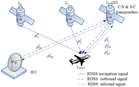
In order to determine user position $(x_{u}, y_{u}, z_{u})$ in three dimensions, measurements are made to at least three satellites S₁, S₂ and S₃ by user receiver. More specifically, at any epoch $t_{k}$ , the pseudorange difference $Δ ρ_{L}^{i, j} (t_{k}) = ρ_{L}^{i} (t_{k}) - ρ_{L}^{1} (t_{k})$ ( $i$ and $j$ are the satellite PRN number of Compass, $i \neq j$ , and $j$ is limited to a visible GEO PRN number, for example, $j =$ 1 is assumed here), and $ρ_{s}^{1} (t_{k})$ are measured. Meanwhile, $ρ_{s}^{1} (t_{k})$ is assumed to be consistent with the pseudorange $ρ_{L}^{1} (t_{k})$ after calibrated ionosphere errors caused by different frequencies between RDSS S and RNSS L using MCC precision ephemeris, ionosphere model parameters. As soon as observations are accomplished, the user receiver transmits to MCC using a transmission burst through inbound channel in response to a message request. The transmission parameters would include all the $Δ ρ_{L}^{i, 1} (t_{k})$ . It is noted that the actual measurements are $ρ_{L D}^{1}$ and $Δ ρ_{L}^{i, 1}$ . Hence, in the absence of measurement errors, the basic set of positioning equations and the geometry matrix $H$ can be expressed as:

1

\{\begin{array}{l} ρ_{L D}^{1} = f (ρ_{C U}^{1} + ρ_{S}^{1} + ρ_{L U}^{1} + ρ_{C D}^{1}) = f (x_{u}, y_{u}, z_{u}), \\ Δ ρ_{L}^{2,1} = ρ_{L D}^{2} - ρ_{L D}^{1}, \\ \dots \\ Δ ρ_{L}^{n, 1} = ρ_{L D}^{n} - ρ_{L D}^{1}, \end{array}

2

H = [\begin{matrix} \frac{\partial F_{1}}{\partial x_{u}} & \frac{\partial F_{1}}{\partial y_{u}} & \frac{\partial F_{1}}{\partial z_{u}} \\ \frac{x_{2} - x_{u}}{r_{2}} - \frac{\partial F_{1}}{\partial x_{u}} & \frac{y_{2} - y_{u}}{r_{2}} - \frac{\partial F_{1}}{\partial y_{u}} & \frac{z_{2} - z_{u}}{r_{2}} - \frac{\partial F_{1}}{\partial z_{u}} \\ . . . & \dots & . . . \\ \frac{x_{n} - x_{u}}{r_{n}} - \frac{\partial F_{1}}{\partial x_{u}} & \frac{y_{n} - y_{u}}{r_{n}} - \frac{\partial F_{1}}{\partial y_{u}} & \frac{z_{n} - z_{u}}{r_{n}} - \frac{\partial F_{1}}{\partial z_{u}} \end{matrix}],

where $F_{1} (\cdot)$ in Eq. (2) is the nonlinear observation function, $ρ_{L D}^{I}$ is the pseudorange to the $i$ ^th satellite, $Δ ρ_{L}^{i, 1}$ is the RNSS pseudorange difference between the $i$ ^th satellite and GEO satellite. The sum of $ρ_{C U}^{1}$ , $ρ_{S}^{1}$ , $ρ_{L U}^{1}$ and $ρ_{C D}^{1}$ are MCC-satellite-user back and forth pseudorange measurements. $(x_{u}, y_{u}, z_{u})$ and $(x_{i}, y_{i}, z_{i})$ denote the user position and $i$ ^th satellite 3-D position, respectively.

If measurements can be modeled accurately and there are no other measurement errors, the linearized equations for CRDSS can be written as follows. For convenience, two new variables are defined as follows:

3

Δ O = [\begin{matrix} Δ ρ_{L D}^{1} \\ Δ (Δ ρ_{L}^{2}) \\ Δ (Δ ρ_{L}^{3}) \end{matrix}], Δ x = [\begin{matrix} Δ x_{u} \\ Δ y_{u} \\ Δ z_{u} \end{matrix}],

where $(Δ x_{u}, Δ y_{u}, Δ z_{u})$ are perturbations in $(x_{u}, y_{u}, z_{u})$ , and the $Δ O$ are the resulting perturbations in the pseudoranges. Therefore, Eq. (1) can be rewritten using matrix notation as:

4

Δ O = H Δ x,

where $(Δ x_{u}, Δ y_{u}, Δ z_{u})$ is displacedment in $(x_{u}, y_{u}, z_{u})$ , and the $Δ O$ are the resulting displacedments in the pseudoranges.

If the pseudorange errors are Gaussian and the covariance of UEREs for the visible satellites is given by the matrix $R_{ρ}$ , then the optimal solution for user position is obtained by iterating:

5

Δ x = {[H^{T} R_{ρ}^{- 1} H]}^{- 1} H^{T} R_{ρ}^{- 1} Δ ρ,

where $R_{ρ}$ is the covariance matrix associated with the measurement errors, the resulting error covariance matrix $P_{x}$ for $Δ x$ is:

6

P_{x} = {[H^{T} R_{ρ}^{- 1} H]}^{- 1} σ_{U E R E}^{2} .

3. Simulation model

3.1. Architecture of simulator

Consider the architecture and the simulation algorithm. Compass dual-mode simulator simulates satellite and receiver trajectories, signal measurement errors and receiver measurement errors. The simulator consists of two main parts. The first one is the signal parameter calculation unit which calculates observation data according to the satellite orbit model, the target trajectory calculation model and the signal propagation error model. The second one is signal generator unit, which uses observation data to generate RF navigation signal.

Fig. 2A schematic graph show Compass dual-mode simulator’s composing

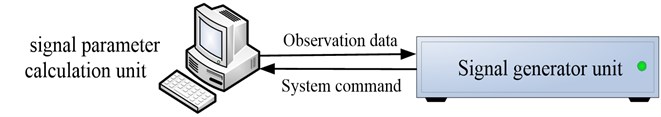
Fig. 3Compass dual-mode simulator flowchart

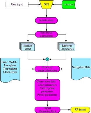
Fig. 4Pseudorange calculation flowchart

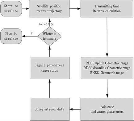
Fig. 3 and Fig. 4 further describe the details on the architecture and flowchart of the simulator. The GUI interface allows the user to set/input various parameters, such as constellation parameters, simulation start time, receiver trajectory, environment error, effects, etc. The simulator uses special orbit integration or interpolation techniques for the computation of the satellite positions. For a realistic modelling of the measurements, signal propagation effects, such as ionosphere, troposphere and delays due to errors caused by the satellites are simulated. As an output either pseudorange and navigation data or a RF signal is provided to the user receiver.

The Compass dual-mode simulator designed in the paper consist of four simulation models, signal transmitting time iterative model, satellite orbit approximation model, signal propagation delay model and the target trajectory calculation mode, which are summarized in Table 1. For a limited length of the paper, the first two models would be analyzed and established in the following sections.

Table 1Error models of passive location

Model	The reason for simulation
Signal transmitting time iterative model	Determine the signal transmitting time for RNSS, and the signal transmitting and retransmitting time for RDSS.
Satellite orbit approximation model	Calculate satellite orbit parameter (position, velocity, acceleration) at the transmitting or retransmitting time.
Signal propagation delay model	Generate pseudorange errors using ionosphere troposphere and relativistic effect modes, respectively.
Target trajectory calculation model	Simulate receiver position, velocity, acceleration, jerk.

3.2. Signal transmitting time iterative model

According to the principle of position determination, the signal received by the receiver at time $t_{r}$ is transmitted by the satellite at time $t_{t}$ . In order to simulate the signal appropriately, the satellite position and the delay should be calculated iteratively. Therefore, obtaining the time $t_{t}$ when the satellite transmits the signal is the key point of the algorithm. As an example of how to use the model to calculate time, the process of calculating $t_{t}$ is given as follows.

Assuming $t_{t}$ is expressed in BDT. $r$ is the geometric satellite-to-receiver distance. $c$ is the speed of light in vacuum. Then the transmitting time is calculated as:

7

t_{t} = t_{r} - \frac{r}{c} - I - T - τ_{s a g},

where $I$ is the ionospheric delay, $T$ is the tropospheric delay, and $τ_{s a g}$ is the delay caused by the earth rotation.

Given the geometric range $r$ is computed in a CGCS2000 coordinate frame. $t_{t}$ ( $k + 1$ ) is the transmitting time calculated iteratively by $k + 1$ times. The initial value is $t_{t} = t$ and the iteration finishes when Eq. (8) condition is satisfied:

8

|r (t_{s} (k + 1)) - r (t_{s} (k))| < ε,

where $ε$ denotes the precision, and it is always equal to or less than 10e-10. Simulation shows that in the condition of $ε =$ 1e-10, the calculation will converge in 3 ~ 4 iterative times and, therefore, $t_{t}$ ( $k + 1$ ) is the signal transmitting time.

3.3. Efficient satellite orbit approximation model

Since the broadcast ephemeris is used to determine satellite positions, orbital errors must be simulated, which would affect the navigation accuracy directly.

Given ephemeris, the best estimate is achieved by directly calculating the satellite’s position and velocity from the model. Howerver, a major issue for a realistic signal modelling is the computation of the Keplerian orbit parameters including their correction terms based on the simulated orbits is a crucial task, since they have to fulfill specific accuracy of navigation solution. So in order to speed up position and velocity computation and get good quality of satellite position and velocity estimates, orbit interpolation is an appropriate method. Among many interpolation methods, the 3^rd-order Hermit interpolation has high efficiency in both position and velocity [11]. For a detailed description of the Hermit interpolation algorithm refer to [12]. In general, Hermit interpolation can be set up as:

9

H (t) = a_{i} + b_{i} (t - t_{i}) + c_{i} {(t - t_{i})}^{2} + d_{i} {(t - t_{i})}^{3},

10

a_{i} = f (t_{i}),

b_{i} = f^{'} (t_{i}),

c_{i} = \frac{3 f [t_{i}, t_{i + 1}] - 2 f^{'} (t_{i}) - f^{'} (t_{i + 1})}{t_{i + 1} - t_{i}},

d_{i} = \frac{f' (t_{i}) - 2 f [t_{i}, t_{i + 1}] + f' (t_{i + 1})}{{(t_{i + 1} - t_{i})}^{2}},

where $t_{i}$ is the sample instants, and they are assumed to be in strictly increasing order, i.e., $t_{i} < t_{i} + 1$ for all $i$ . $H (t)$ is the function evaluated at value $t$ . $a_{i}$ , $b_{i}$ , $c_{i}$ and $d_{i}$ are the coefficients of the polynomial. $f (t)$ is Hermite polynomial and $f' (t)$ is the derivative of $f (t)$ , in our case is the ECEF satellite position and velocity coordinate $X$ , $Y$ or $Z$ , respectively.

Here 1-min interval sampled data for the time span from 04 h through 24 h of 2007-09-06 is calculated from RNSS navigation message ephemeris. Then sampled data is subdivided into two 2-minute interval observation data. One is used for sampling instants, the other is developed as the reference sampled data.

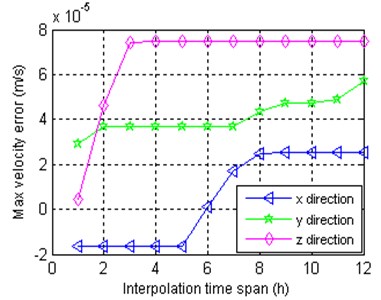
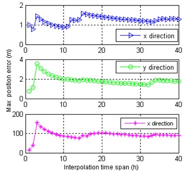
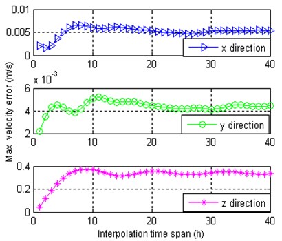
It can be seen in Fig. 5 that for reasonable position error of 5-15 mm and velocity error of 4-6 mm/s, the shorter interpolation time span, the more efficient of Hermit interpolation algorithm. In Fig. 6, a comparison with 40 hour RDSS observation data are provided, which has larger errors. So piecewise polynomial interpolation is needed for long interpolation area [11]. In order to validate the precison, the comparisons among GEO, IGSO and MEO with above data for time span from 04 h through 05 h are made, as shown in Fig. 7 and Fig. 8.

From the summary in Table 2, for either satellite type, the precision is less than 1e-2 m and 1e-5 m/s. Therefore, the effect on navigation solution can be neglected.

Fig. 5Max. error of MEO satellite position and velocity vs. different time span, using RNSS ephemeris from navigation message

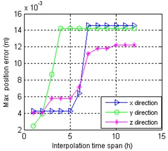
a) Postion error

b) Velocity error

As a conclusion, Hermit interpolation reduces the cost of satellite location and velocity determination remarkably, also satisfies orbit approximation curevs’s continuity, precision requirements. So the Hermit interpolation is appropriate for navigation satellite orbit calculating, also a compromise between computational burden and precision.

Fig. 6Max. error of GEO satellite position and velocity vs. different time span, using RDSS broadcast information

a) Postion error

b) Velocity error

Fig. 7Position error vs. different satellite types

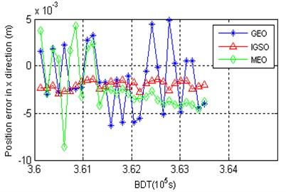
Fig. 8Velocity error vs. different satellite types

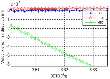
Fig. 9A schematic graph shows Compass dual-mode simulation system

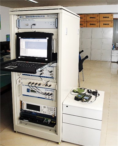
Table 2Precision of different type satellite with Hermit interpolation (m)

Sat. Type	Max error		Min error		RMS error
Sat. Type	Position	Velocity	Position	Velocity	Position	Velocity
GEO	6.303e-3	1.097e-6	1.424e-4	1.355e-8	3.512e-5	5.114e-9
IGSO	2.913e-3	2.678e-5	1.431e-3	1.736e-6	2.113e-5	2.452e-8
MEO	8.604e-3	6.916e-5	6.850e-4	1.6534e-5	3.692e-5	4.784e-7

4. Experiments and analysis

4.1. System design and implementation

Considering the dual-mode receiver test requirements, the Compass dual–mode simulator integration with evaluation function shows in Fig. 9 is designed and implemented to support all types of BD receivers. The key performance for user is shown here:

1. Pseudorange accuracy: ±0.003 m.

2. Rate of pseudorange accuracy change rate: ±0.003 m/s.

3. Channel delay stability: 0.167 (code) ≤ 0.001 m (carrier).

4. Equipment delay stability: 1 ns/month.

4.2. Experimental results

In evaluating the performance of the dual-mode receiver, we are interseted in two simulator-based experiments, the dynamic position accuracy and the difference pseudorange, are carried out. Experiments are conducted in cable connect environment based on the above navigation receiver integrated test system, as shown in Fig. 9, which consists of Compass dual simulator and a prototype receiver with CRDSS.

In the experiment, the simulation beginning time of scenarios is at 314 BD week number and 3.6e4 second of week, the constellation configure is Compass (Phase I), the rate of observation data is set to 1 Hz, and the average number of visible satellites is 7. It should be noted that the second experiment’s observation data is the difference pseudorange measurement only, without MCC-satellite-user back and forth pseudorange measurements. For the receiver is unable to simulate the signal arriving at MCC’s antenna with actual pseudorange in the simulation environment. If pseudorange measured from the receiver inbound signal, large error will be caused which, furthermore, affected the navigation solution’s reality. Therefore, limited the simulation environment, the position fixing and report of the receiver can be only assessed indirectly by measuring difference pseudorange.

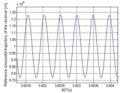
Equation (11) is the trajectory expression of the dynamic position accuracy scenario, which is a sinusoidal movement curve in the altitude direction of geodetic coordinates. The center position is set to (40°N, 112°E, 1000 m), which is shwon in Fig. 10:

11

s = s_{0} + A s i n (w t + ϕ),

where $s$ is the real time pseudorange from satellites. $s_{0}$ is the initial pseudorange determined by the initial user receiver position. $A$ is a constant amplitude with a value 2296 m. Angular frequency $ω$ is set to 0.1307 rad/s. The initial phase $φ$ is zero rad.

Fig. 10Experimental receiver true trajectory

Furthermore, Fig. 11, Fig. 12, Fig. 13, Fig. 14 and Table 3 present the test result of the dynamic position and velocity accuracy in different direction by RNSS alone solution, which is in accordance with the one provided by Compass. It can be noted that there is a pseudorange jump during the test, which is caused by the receiver itself through comparion test with other receivers under the same scenario.

As shown in Fig. 15, Fig. 16, Fig. 17 and Table 4, the accuracy of the difference pseudorange and double zero value is less than 0.1 ns and 1 ns, respectively. That is, the accuracy of comprehensive RDSS position fixing and report would be improved when compared with RDSS standalone solutions and, also better than RNSS by using MCC precision ephemeris, ionosphere model parameters. Furthermore, all the test result proves the signal simulator can satisfy dual-mode receiver’s test requirements completely.

Fig. 11Horizontal positioning errors

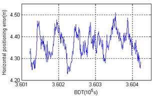
Fig. 12Vertical positioning errors

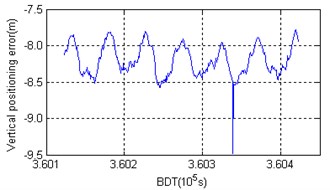
Fig. 13Positioning errors in distance

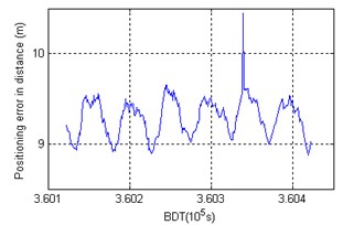
Fig. 143-D dimensional velocity error

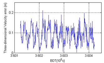
Table 3Accuracy of dynamic position and velocity test

Item	RMS error (m)
Item	Horizontal	Vertical	Distance	Max	Min
Position error	4.374	8.217	9.309	10.446	8.877
Velocity error	--	--	0.099	0.210	0.002

Fig. 15Different pseudorange vs. time

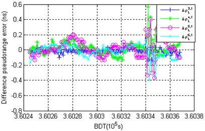
Fig. 16Different pseudorange vs. time

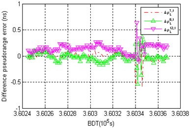
Fig. 17RDSS double zero vs. time, with mean value of 1.001e6 ns and variance of 1.1787 ns

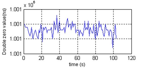
Table 4Difference pseudorange accuracy of CRDSS position fixing and report

Difference pseudorange	$Δ ρ_{L}^{3,1}$	$Δ ρ_{L}^{4,1}$	$Δ ρ_{L}^{5,1}$	$Δ ρ_{L}^{6,1}$	$Δ ρ_{L}^{7,1}$	$Δ ρ_{L}^{8,1}$	$Δ ρ_{L}^{12,1}$
RMS error (ns)	0.0360	0.095	0.122	0.0856	0.0968	0.107	0.165

5. Conclusions

As a conclusion, the simulation models are proposed and analyzed based on the dual-mode receiver’s test requirements. The discussion here focuses on the transmitting time iterative model, satellite orbit approximation model and the ways to improve model accuracy. Finally, the implementation of the simulator and the analysis of the two simulator-based experimental result with the prototype receiver are given. Compared with the existing simulator, the Compass dual-model simulator can simulate the RDSS and RNSS signal simultaneously to support all types of BD receiver’s performance evaluation, such as RDSS, RNSS and dual-mode receiver. The test results indicate that the accuracy of position and velocity is 9.3 m and 0.099 m/s, respectively. Even more importantly, the function of CRDSS can also be validated, with the accuracy of difference pseudorange and double zero value less than 0.1 ns and 1 ns. Therefore, the Compass dual-model’s design completely meets the test requirements.

References

Jämasä J., Luimula M., Pieskä S., Saukko O. Indoor positioning using symmetric double-sided two-way ranging in a welding hall. Journal of Vibroengineering, Vol. 14, Issue 1, 2009, p. 27-30.

Search CrossRef
Winkel J., Wolf R., Prokoph G., Mocker G. The Merlin signal generator – a powerful, low-cost constellation Galileo/GPS signal simulator. Proceedings of the 19th International Technical Meeting of the Satellite Division of the Institute of Navigation (ION GNSS 2006), Fort Worth, TX, September 2006, p. 246-250.

Search CrossRef
Heinrichs G., Irsigler M., Wolf R., Winkel Jon, Prokoph G. NavX(R) – NCS – the first Galileo/GPS full RF navigation constellation simulator. Proceedings of the 20th International Technical Meeting of the Satellite Division of the Institute of Navigation (ION GNSS 2007), Fort Worth, TX, September 2007, p. 1323-1328.

Search CrossRef
Artaud G., De Latour A., Dantepal J., Ries L., Maury N., Denis J.-C., Senant E., Bany T. A new GNSS multi constellation simulator: NAVYS. Proceedings of the 23rd International Technical Meeting of the Satellite Division of the Institute of Navigation (ION GNSS 2010), Portland, OR, September 2010, p. 845-857.

Search CrossRef
Li R., Zeng D. Z. Long T., Zhang L. Architecture and implementation of a universal real-time GNSS signal simulator. Proceedings of the 2010 International Technical Meeting of the Institute of Navigation, San Diego, CA, January 2010, p. 1037-1043.

Search CrossRef
Berglez P., Wasle E., Seybold J., Hofmann-Wellenhof B. GNSS constellation and performance simulator for testing and certification. Proceedings of the 22nd International Technical Meeting of the Satellite Division of the Institute of Navigation (ION GNSS 2009), Savannah, GA, September 2009, p. 2220-2228.

Search CrossRef
Li G. F., Zhu M. C. The study of real-time simulation for the radio determination satellite service (RDSS). Modeling and Simulation in Distributed Applications, Changsha, CA, 2001, p. 721-725.

Search CrossRef
Zhang G. H., Sun C. Y. Simulation and implementation of BD-1 dynamic navigation signals. Journal of System Simulation, Vol. 17, Issue 11, 2005, p. 2731-2733.

Search CrossRef
China Satellite Navigation Office. Development of BeiDou navigation satellite system. Proceedings of the 23rd International Technical Meeting of the Satellite Division of the Institute of Navigation (ION GNSS 2011), Portland, USA, 2011.

Search CrossRef
Tan S. S. Theory and application of comprehensive RDSS position and report. Acta Geodaetica et Cartographica Sinica, Vol. 38, Issue 1, 2009, p. 1-5.

Search CrossRef
Johnson L. J., Riess R. D. Numerical Analysis. Addison-Wesley Publishing Company, Massachusetts, 1982.

Search CrossRef
Tong H. B., Sha H., Zhang G. Z., Ou G. A high-precision and real-time interpolation method for satellite orbit in GNSS. Journal of Navigation, University of Defense Technology, Vol. 34, Issue 2, 2012, p. 59-63.

Search CrossRef

About this article

Received

02 February 2013

Accepted

03 June 2013

Published

30 June 2013

Keywords

BeiDou navigation satellite system (Compass/BDS)

signal simulator

Hermit interpolation

dual-mode receiver

test

This is an open access article distributed under the Creative Commons Attribution License, which permits unrestricted use, distribution, and reproduction in any medium, provided the original work is properly cited.